Data Cleaning with Pandas

2. Tidy Data

2.1 📊 What is Tidy Data?
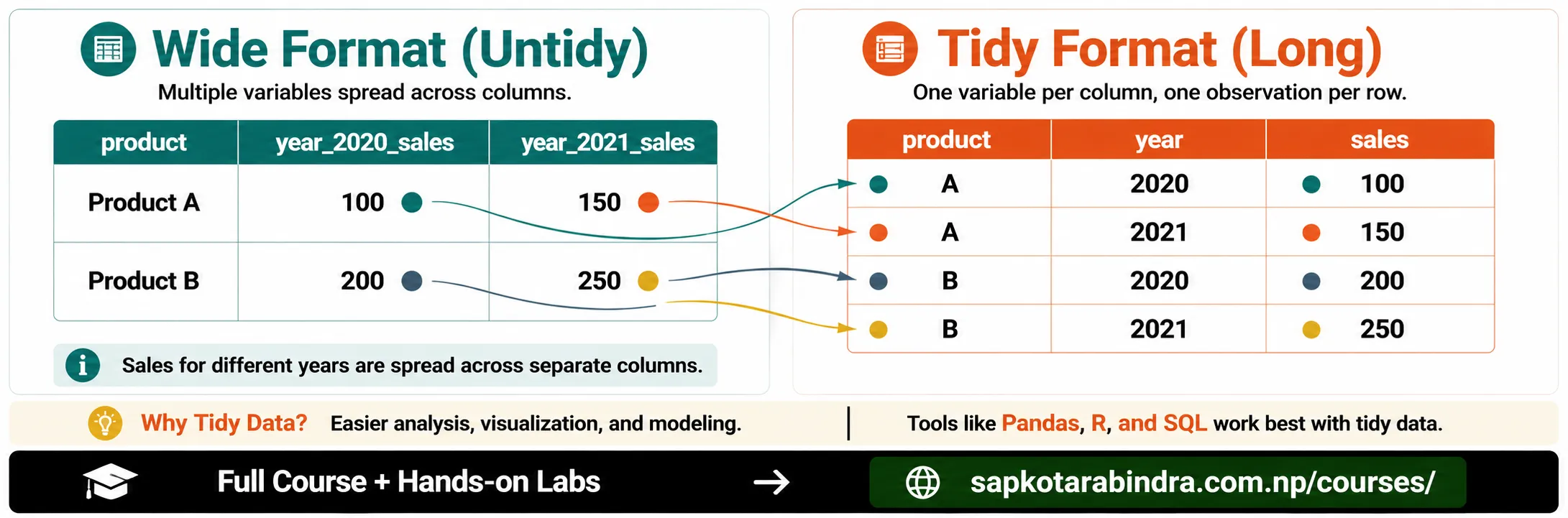
1. Tidy data is a standard way of organizing data for analysis. In tidy data: ✅ Each variable forms a column ✅ Each observation forms a row ✅ Each type of observational unit forms a table 📌 Simple idea: Tidy data is organized data that is easier to analyze.
2.2 Example of Untidy Data
1. Here, sales for different years are stored in different columns.

2.3 Example of Tidy Data
1. Here: - product is a column - year is a column - sales is a column - Each row is one observation 📌 Tidy data is usually better for analysis. Wide data is often better for reporting.

3. melt()

3.1 🔄 What is melt()?
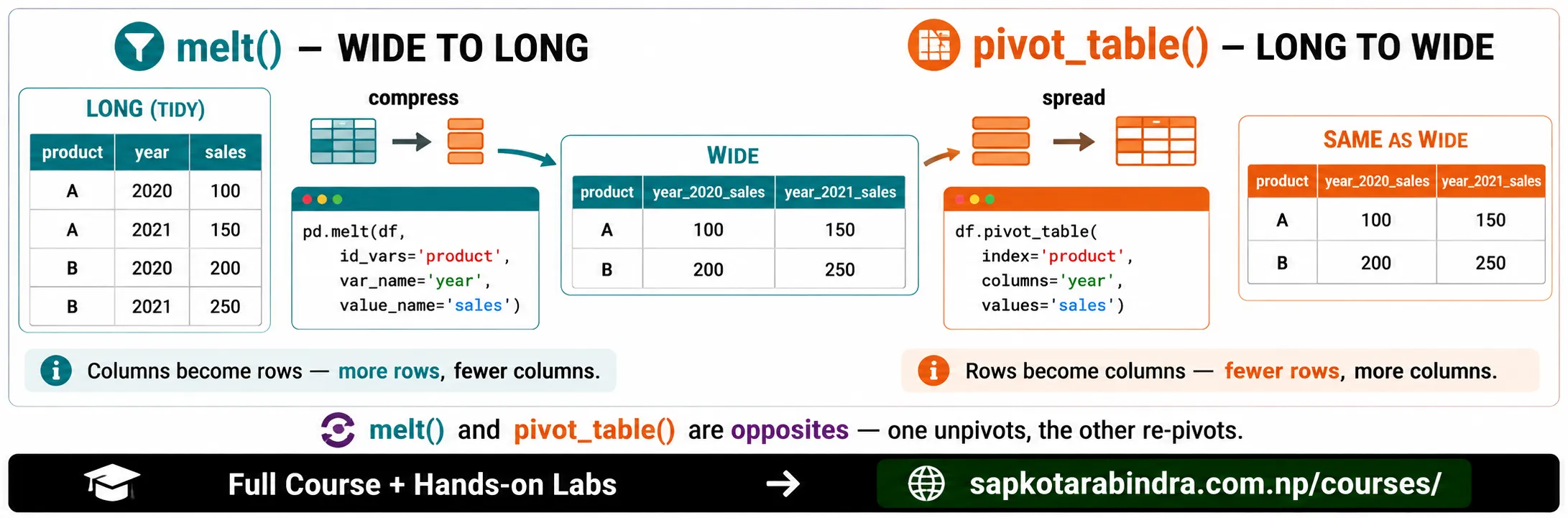
1. melt() converts data from wide format to long format. This is useful when we want to convert untidy data into tidy data. 📌 Simple idea: melt() turns many value columns into two columns: variable and value.
3.2 What Happens During Melt?
1. When we use melt(): - Number of rows usually increases - Number of columns usually decreases
3.3 Syntax
1. pd.melt(df,id_vars=["id_1", "id_2"],value_vars=["val_1", "val_2"] ) Here: id_vars are columns we want to keep fixed value_vars are columns we want to unpivot
3.4 Example: Melt Sales Data
1. import pandas as pddf = pd.DataFrame({"product": ["A", "B"],"year_2020_sales": [100, 200],"year_2021_sales": [150, 250] })melted_df = pd.melt(df,id_vars=["product"] )print(melted_df)Output: product variable value 0 A year_2020_sales 100 1 B year_2020_sales 200 2 A year_2021_sales 150 3 B year_2021_sales 250
3.5 Better Column Names After Melt
1. melted_df = pd.melt(df,id_vars=["product"],var_name="year",value_name="sales" )print(melted_df) 📌 var_name gives a name to the old column-name column. 📌 value_name gives a name to the value column.

4. pivot_table()

4.1 📌 What is pivot_table()?
1. pivot_table() converts data from long format to wide format. It is like the reverse of melt(). 📌 Simple idea: pivot_table() spreads values into separate columns.
4.2 What Happens During Pivot?
1. When we use pivot_table(): - Number of rows usually decreases - Number of columns usually increases
4.3 Syntax
1. df.pivot_table(index=["id_1", "id_2"],columns="variable",values="value" )
4.4 Handling Duplicate Values
1. If there are duplicate values for the same index and column combination, pivot_table() aggregates them. By default, it uses average. We can change this using aggfunc. Example: df.pivot_table(index="product",columns="year",values="sales",aggfunc="sum" )
4.5 Example: Pivot Sales Data
1. import pandas as pddf = pd.DataFrame({"product": ["A", "A", "B", "B"],"year": [2020, 2021, 2020, 2021],"sales": [100, 150, 200, 250] })p_df = df.pivot_table(index="product",columns="year",values="sales" )print(p_df)Output: year 2020 2021 product A 100 150 B 200 250

5. cut() and qcut()

5.1 ✂️ What is cut()?
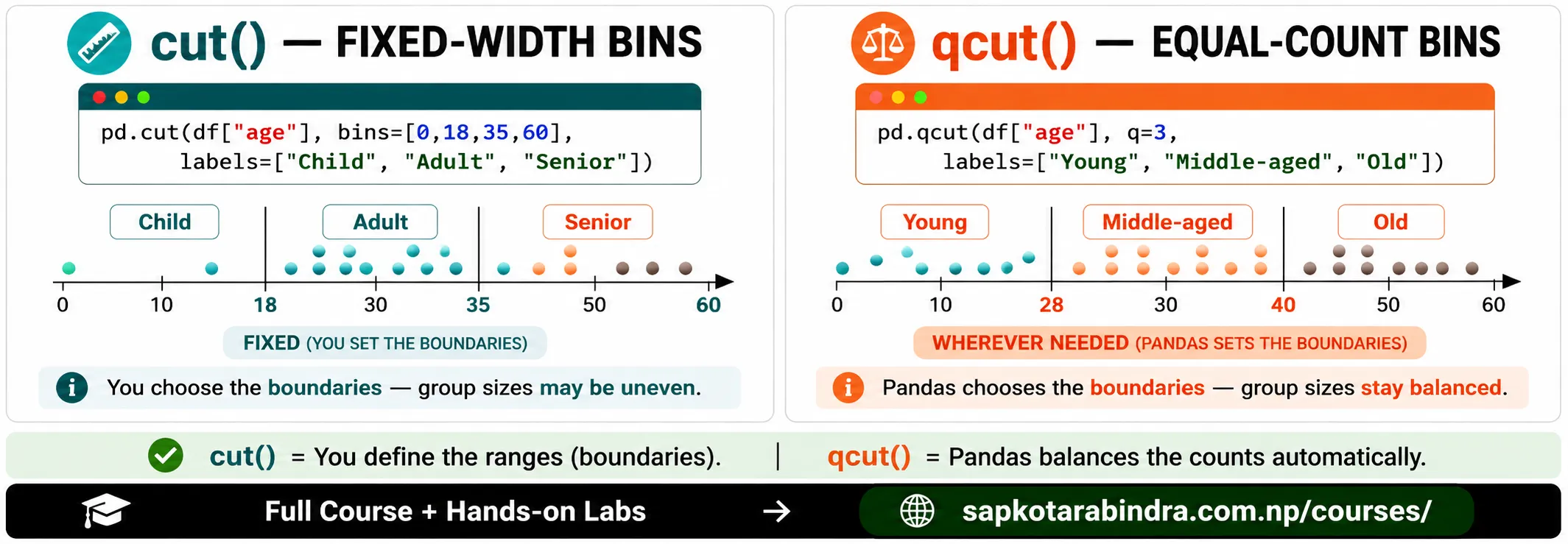
1. cut() is used to divide numeric values into bins based on fixed ranges. Example: 0 to 18 = Child 18 to 35 = Adult 35 to 60 = Senior
5.2 Example: cut()
1. bins = [0, 18, 35, 60] labels = ["Child", "Adult", "Senior"]df["age_group"] = pd.cut(df["age"],bins=bins,labels=labels )print(df) 📌 cut() uses the bin limits we provide.
5.3 What is qcut()?
1. qcut() divides data into equal-sized groups based on quantiles. Example: If we use: q=3 Pandas tries to divide the data into 3 groups with similar number of rows.
5.4 Example: qcut()
1. labels = ["Young", "Middle-aged", "Old"]df["age_quantile"] = pd.qcut(df["age"],q=3,labels=labels )print(df) 📌 Simple idea: cut() uses fixed ranges. qcut() uses quantiles.

6. Handling Missing Values

6.1 ❓ What are Missing Values?
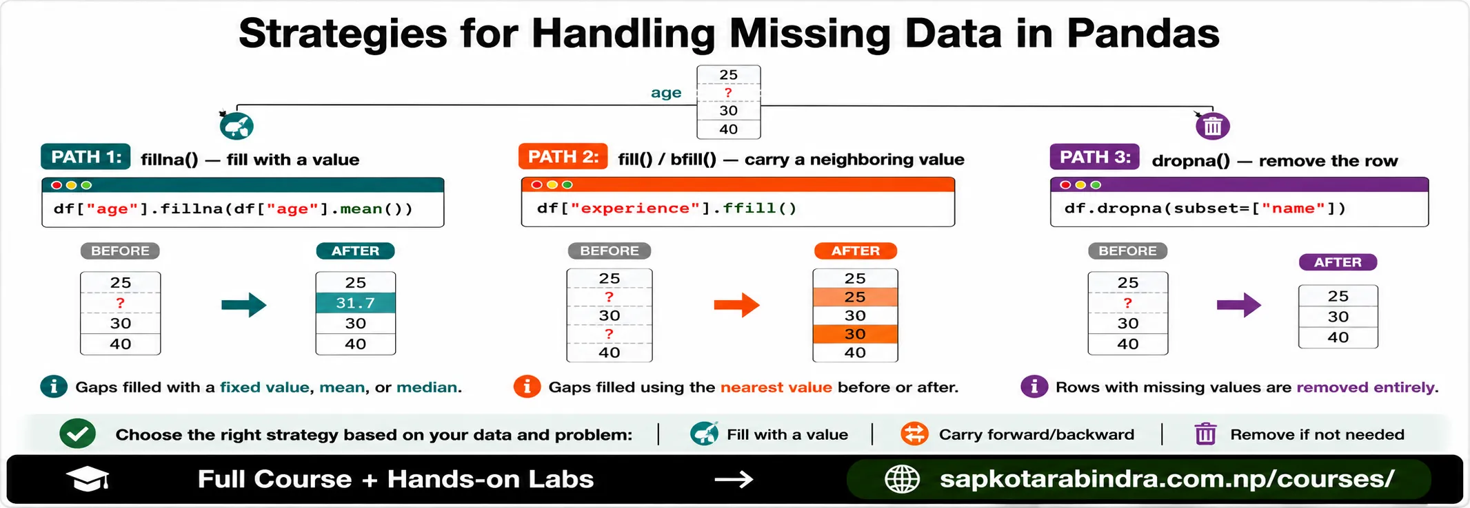
1. Missing values are empty or unknown values in data. In Pandas, missing values are often shown as: NaN Common strategies: ✅ Drop missing rows or columns ✅ Fill missing values with a fixed value ✅ Fill missing values using mean, median, or mode ✅ Use forward fill or backward fill ✅ Estimate missing values using interpolation or prediction
6.2 Fill Missing Text Values
1. df["course_clean"] = df["course"].fillna("Unknown") This replaces missing course values with "Unknown".
6.3 Fill Missing Numeric Values
1. df["age_clean"] = df["age"].fillna(df["age"].mean()) This replaces missing age values with the average age.
6.4 Forward Fill
1. df["experience_clean"] = df["experience"].ffill() This fills missing values using the previous available value. Backward fill: df["experience_clean"] = df["experience"].bfill()
6.5 Fill Missing Values with Conditions
1. filter_mask = (df["education"].isnull()) & (df["age"] < 25)df.loc[filter_mask, "education"] = "SLC" This fills missing education values with "SLC" only when age is below 25.
6.6 Drop Rows with Missing Values
1. df.dropna(subset=["name"], inplace=True) This removes rows where name is missing. 📌 Use fillna() when you want to fill missing values. 📌 Use dropna() when you want to remove missing rows.

7. Handling Duplicates

7.1 👥 What are Duplicates?
1. Duplicate rows are repeated records in a dataset. They can happen due to: - Repeated data entry - Multiple file imports - System errors - Merged data from different sources
7.2 Find Duplicate Rows
1. duplicate_mask = df.duplicated(subset=["name", "age"],keep=False )duplicates = df[duplicate_mask]print(duplicates) Here: subset=["name", "age"] checks duplicates using these columns keep=False marks all duplicate rows as duplicates
7.3 Remove Duplicate Rows
1. unique_df = df.drop_duplicates(subset=["name", "age"],keep="first" )print(unique_df.duplicated(subset=["name", "age"]).sum()) 📌 duplicated() finds duplicates. drop_duplicates() removes duplicates.

8. Data Value Issues

8.1 🧩 Inconsistent Categories
1. Sometimes the same category is written in different ways. Example: m, male, Male, M We can standardize values using replace(). df["gender"] = df["gender"].replace({"m": "Male","f": "Female" })
8.2 Using map()
1. mapping_dict = {"m": "Male","f": "Female" }df["gender"] = df["gender"].str.lower().map(mapping_dict) 📌 Note: replace() keeps values that are not in the dictionary. map() may convert unmatched values to missing values.
8.3 Outliers
1. Outliers are values that are unusually high or unusually low. Example: Age = 300
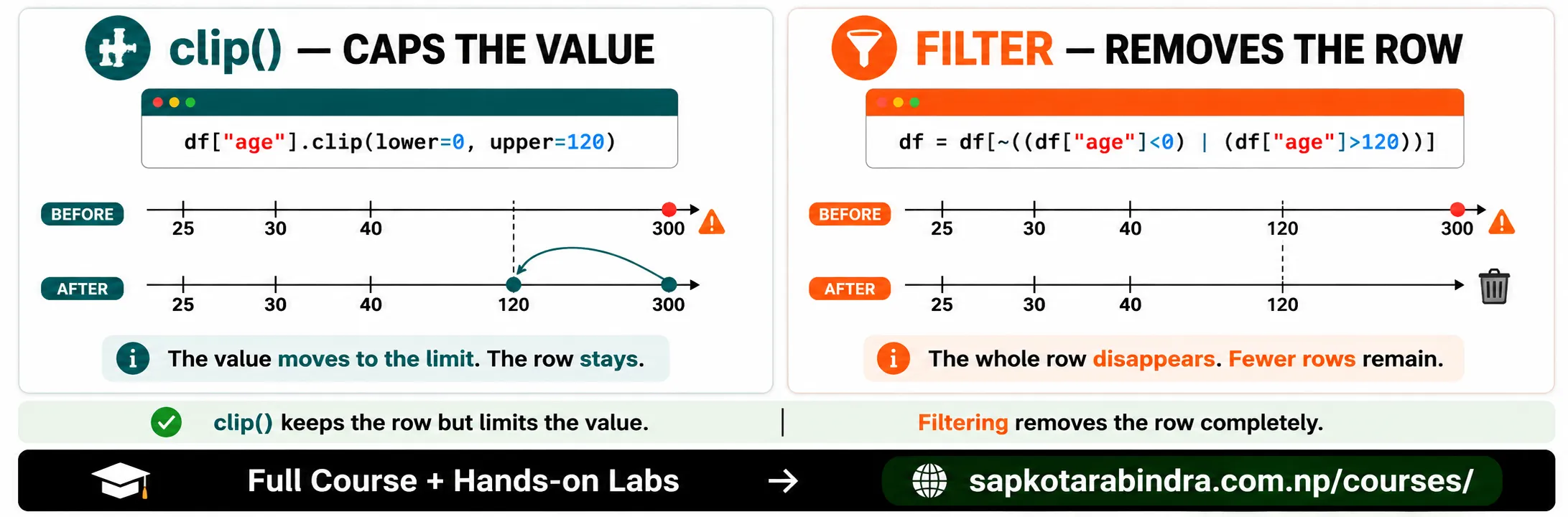
8.4 Limit Outliers with clip()
1. df["age"] = df["age"].clip(lower=0, upper=120) This limits age values to the range 0 to 120.
8.5 Remove Outliers with Filter
1. outlier_mask = (df["age"] < 0) | (df["age"] > 120)df = df[~outlier_mask] This removes rows where age is below 0 or above 120.

8.6 Leading and Trailing Spaces
1. df["name"] = df["name"].str.strip() This removes extra spaces from the beginning and end of names.
8.7 Inconsistent Case
1. df["name"] = df["name"].str.upper() or: df["name"] = df["name"].str.lower() This makes text values consistent.
8.8 Non-Numeric Characters in Numeric Columns
1. Sometimes numeric columns contain characters. Example: "25 years" We can remove non-numeric characters using regex. df["age"] = df["age"].str.replace(r"\D","",regex=True ).astype(int) 📌 Simple idea: Text cleaning often uses .str, replace(), and regex.

9. Fuzzy Matching to Clean Spelling Issues

9.1 🔤 What is Fuzzy Matching?
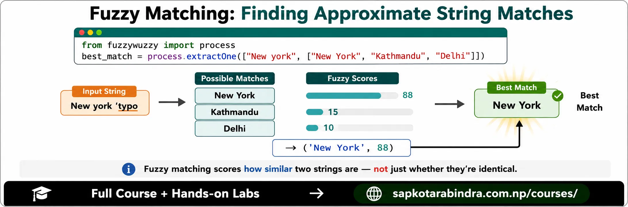
1. Fuzzy matching is used to find strings that are approximately similar, not exactly the same. Example: New yolk ≈ New York It is useful for fixing spelling mistakes or inconsistent location names.
9.2 Library for Fuzzy Matching
1. The fuzzywuzzy library can be used for fuzzy matching in Python. Install it using: pip install fuzzywuzzy python-Levenshtein
9.3 Example: Fuzzy Matching
1. from fuzzywuzzy import processchoices = ["New York", "Kathmandu", "Delhi"]query = "New yolk"best_match = process.extractOne(query, choices)print(best_match)Possible output: ('New York', 88) 📌 The result contains: - Best matching text - Similarity score 📌 Simple idea: Fuzzy matching helps clean values that are close but not exactly the same.