
DataFrame Operations
✕1. Index Operations
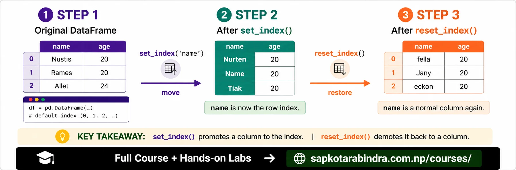
- An index is used to label rows in a DataFrame. By default, Pandas gives rows a numeric index:
0, 1, 2, 3, ...But we can also set a column as the index. 📌 Simple idea: An index helps Pandas identify rows. - We can use
set_index()to make a column the index.df.set_index("name", inplace=True)print(df)Here, the name column becomes the row index. - We can use
reset_index()to bring the index back as a normal column.df.reset_index(inplace=True)print(df)If we want to remove the index completely instead of keeping it as a column:df.reset_index(drop=True, inplace=True)📌set_index()changes the row label.reset_index()brings it back.
1.1 🏷️ What is an Index?
1.2 Set Index
1.3 Reset Index
2. Selecting and Indexing Data
- We can select a single column using:
df["age"]Example:age_series = df["age"]This returns a Series. - We can also write:
df.ageBut this only works when the column name is simple and does not contain spaces or special characters. Recommended style:df["age"]📌df["column"]is safer thandf.column. - To select multiple columns, we pass a list of column names.
sample_df = df[["name", "age"]]📌 Single column ➜ One pair of brackets. 📌 Multiple columns ➜ List inside brackets.
2.1 🎯 Selecting Columns
2.2 Selecting Columns with Dot Syntax
2.3 Selecting Multiple Columns
3. loc and iloc
locselects data using labels. Syntax:df.loc[row_label, column_label]Example:age_loc = df.loc[:, "age"]This selects all rows and the age column.ilocselects data using integer position. Syntax:df.iloc[row_position, column_position]Example:age_iloc = df.iloc[:, 2]This selects all rows and the column at position 2.
3.1 📍 What is loc?
3.2 🔢 What is iloc?
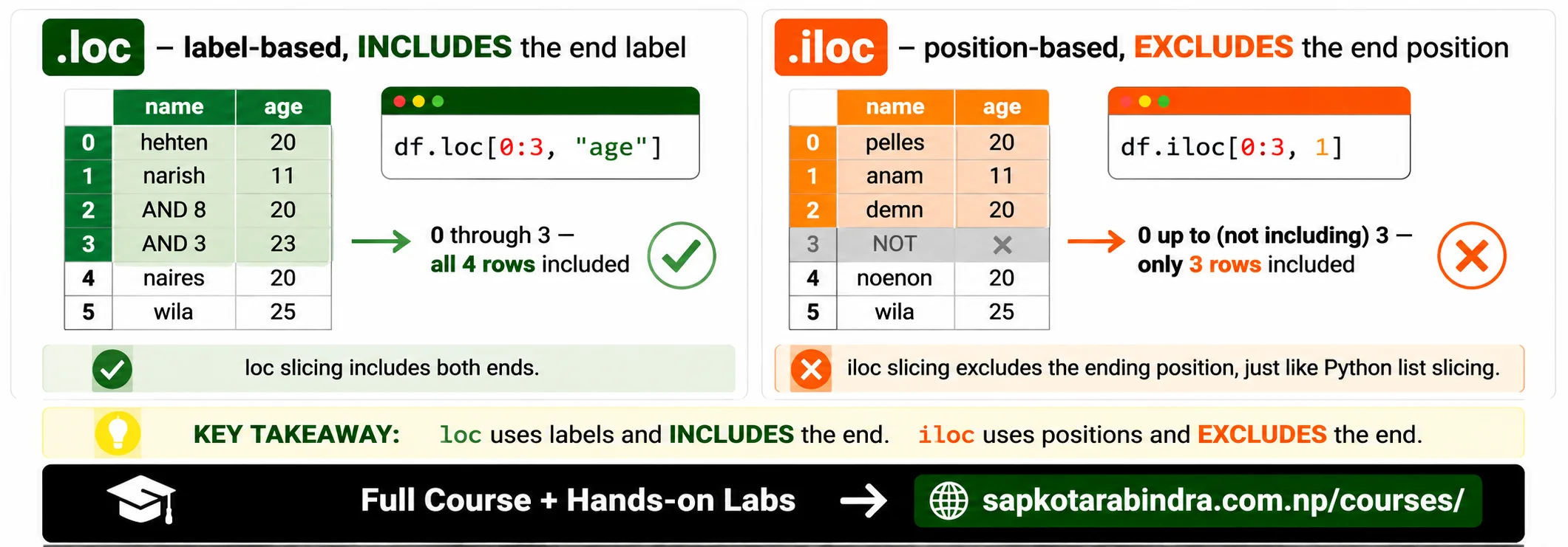
age_series = df["age"]# Select age columnage_loc = df.loc[:, "age"]# Select age column using labelage_iloc = df.iloc[:, 2]# Select column at index position 2sample_df = df[["name", "age"]]sample_loc = df.loc[:, ["name", "age"]]sample_iloc = df.iloc[:, [0, 2]]age_loc_samp = df.loc[0:5, "age"]age_iloc_samp = df.iloc[0:5, 2]age_samp = df["age"][0:5]sample_data = df.loc[0:5, ["name", "age"]]📌locuses labels and includes the ending label in slicing. 📌ilocuses positions and excludes the ending position.
3.3 Selecting Columns Examples
3.4 Selecting Multiple Columns Examples
3.5 Selecting Rows and Columns Together
4. Filtering Data
- Filtering means selecting rows based on a condition. Example: Select people whose age is greater than 30.
age_filter = df["age"] > 30filtered_df = df[age_filter]Shorter version:filtered_df = df[df["age"] > 30]📌 Simple idea: First create a condition. Then use it to filter the DataFrame.- Sometimes we need to use multiple conditions to get the final result. For this, we combine individual conditions using:
&for AND|for OR~for NOT Example:data_filter = (df["age"] > 30) & (df["weight"] < 70)filtered_df = df[data_filter]📌 Always wrap each condition in parentheses. name_filter = df["name"].str.startswith("A")filtered_df = df[name_filter]This selects rows where name starts with A.country_filter = df["country"].isin(["USA", "Canada"])filtered_df = df[country_filter]To exclude those countries:filtered_df = df[~country_filter]📌isin()checks if values are inside a list.
4.1 🔎 What is Filtering?
4.2 Basic Filtering
4.3 Filtering with Multiple Conditions
4.4 Filtering Text Columns
4.5 Filtering with isin()
5. Broadcasting and Vectorized Operations
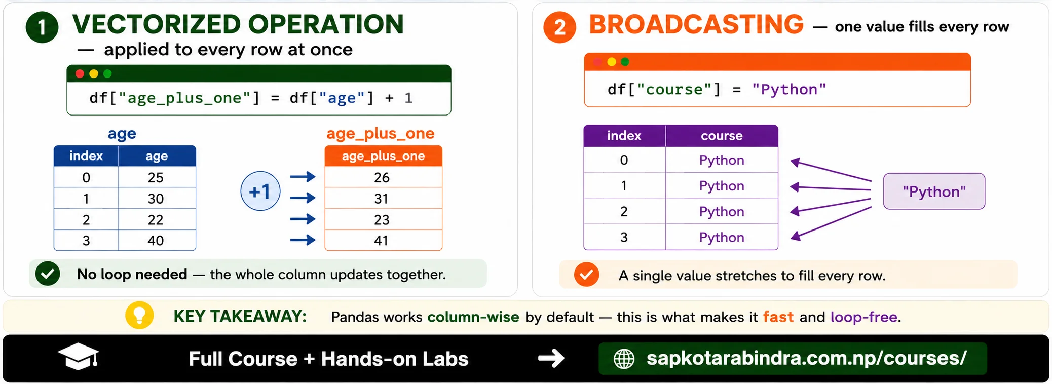
- Pandas operations are usually vectorized. This means operations are applied to the whole column at once instead of using loops.
Example:
df["age_plus_one"] = df["age"] + 1This adds 1 to every value in the age column. 📌 Simple idea: Pandas works column-wise, so we can avoid writing loops. - Broadcasting means assigning one value to many rows.
df["course"] = "Python"This adds a new column where every row has the value "Python". df["age_plus_one"] = df["age"] + 1df["bmi"] = df["weight"] / (df["height"] ** 2)df["is_above_30"] = df["age"] > 30
5.1 ⚡ What are Vectorized Operations?
5.2 Broadcasting Example
5.3 Vectorized Operation Examples
import numpy as nprandom_array = np.random.rand(len(df))df["random_value"] = random_array📌len(df)gives the number of rows in the DataFrame.
5.4 Adding Random Values
6. Sorting and Ranking
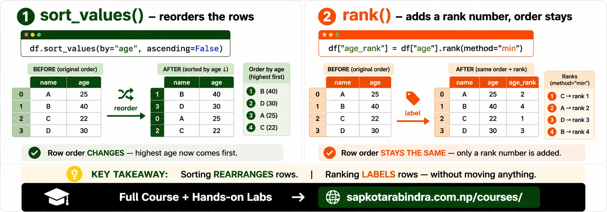
- We can sort a DataFrame using:
sort_values() sorted_df = df.sort_values(by="age", ascending=False)This sorts rows by age from highest to lowest.sorted_df = df.sort_values(by=["age", "weight"],ascending=[True, False])This sorts by: ✅ age in ascending order ✅ weight in descending order- We can create ranks using
rank().ranked_df = df.copy()ranked_df["age_rank"] = ranked_df["age"].rank(method="min")📌 Simple idea: Sorting changes row order. Ranking gives each value a rank number.
6.1 🔃 Sorting Data
6.2 Sort by One Column
6.3 Sort by Multiple Columns
6.4 Ranking
7. Drop and Rename
- We can drop columns using
drop().df_dropped = df.drop(columns=["age", "weight"])Another way:df_dropped = df.drop(["age", "weight"], axis=1)Here,axis=1means column. - We can also drop rows using index labels.
df_dropped = df.drop([0, 1])This drops rows with index labels 0 and 1. - We can rename columns using
rename().df_renamed = df.rename(columns={"age": "Age","weight": "Weight"})📌 Simple idea: Usedrop()to remove rows or columns. Userename()to change column names.
7.1 🗑️ Dropping Columns
7.2 Dropping Rows
7.3 Renaming Columns
8. Concatenating DataFrames
pd.concat()is used to stack DataFrames together. It is similar to adding rows from multiple tables together. Example use case: We have daily sales files and want to combine them into one DataFrame.import pandas as pddf1 = pd.read_csv("2025-01-02.csv")df2 = pd.read_csv("2025-01-03.csv")df3 = pd.read_csv("2025-01-04.csv")combined_df = pd.concat([df1, df2, df3])print(df1.shape)print(df2.shape)print(df3.shape)print(combined_df.shape)
8.1 🧱 What is pd.concat()?
8.2 Example: Combine Multiple CSV Files
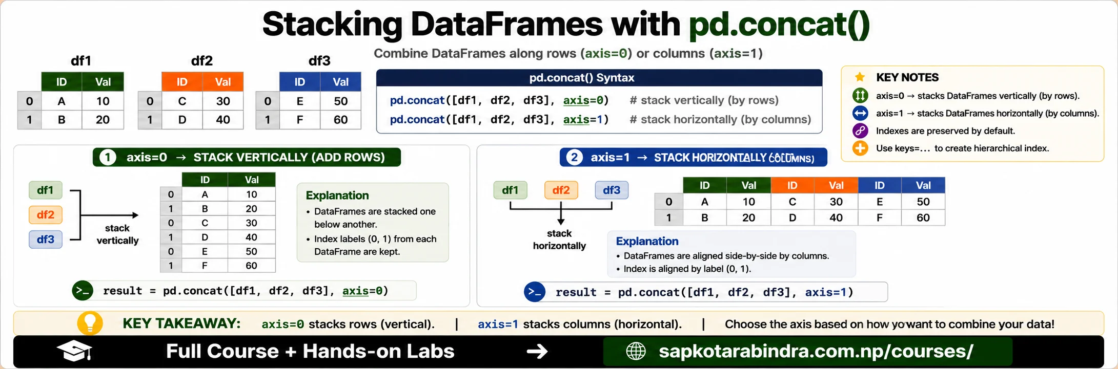
- After concatenation, old indexes may repeat. We can fix that using:
combined_df = pd.concat([df1, df2, df3], ignore_index=True)📌 Simple idea:concat()stacks DataFrames.ignore_index=Truecreates a fresh index.
8.3 Ignore Old Index
9. Merging DataFrames
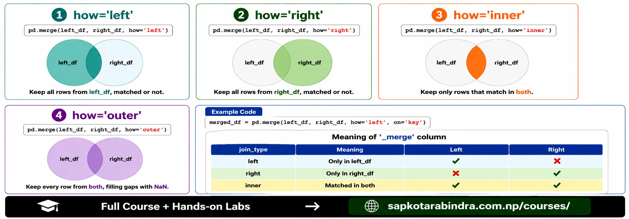
pd.merge()combines DataFrames based on common columns. It is similar to SQL JOIN. Syntax:pd.merge(left_df, right_df, on="key_col", how="left")
9.1 🔗 What is pd.merge()?
9.2 Common how Values
| Value | Meaning |
|---|---|
| left | Keep all rows from left DataFrame |
| right | Keep all rows from right DataFrame |
| inner | Keep only matching rows |
| outer | Keep all rows from both DataFrames |
import pandas as pdleft_df = pd.DataFrame({"customer_id": [1, 2],"name": ["Hari", "Bob"]})right_df = pd.DataFrame({"id": [2, 3],"age": [25, 30]})merged_df = pd.merge(left_df,right_df,left_on="customer_id",right_on="id",how="left")print(merged_df)Output: customer_id name id age 1 Hari NaN NaN 2 Bob 2.0 25.0 📌merge()joins DataFrames using matching key columns. 📌 If both DataFrames have the same key column name, we can use on instead of left_on and right_on.
9.3 Merge Example
10. Data Type Conversion
- Sometimes data is loaded with the wrong data type.
Example:
- Age may load as text
- Date may load as text
- Category may load as normal string
We can convert data types using:
astype()or specialized functions like:pd.to_datetime() df["age"] = df["age"].astype(int)df["weight"] = df["weight"].astype(float)df["name"] = df["name"].astype(str)df["category_col"] = df["category_col"].astype("category")df["date_col"] = pd.to_datetime(df["date_col"])📌 Simple idea: Correct data types make analysis easier and safer.
10.1 🔄 Why Convert Data Types?
10.2 Common Type Conversions
11. GroupBy and Aggregation
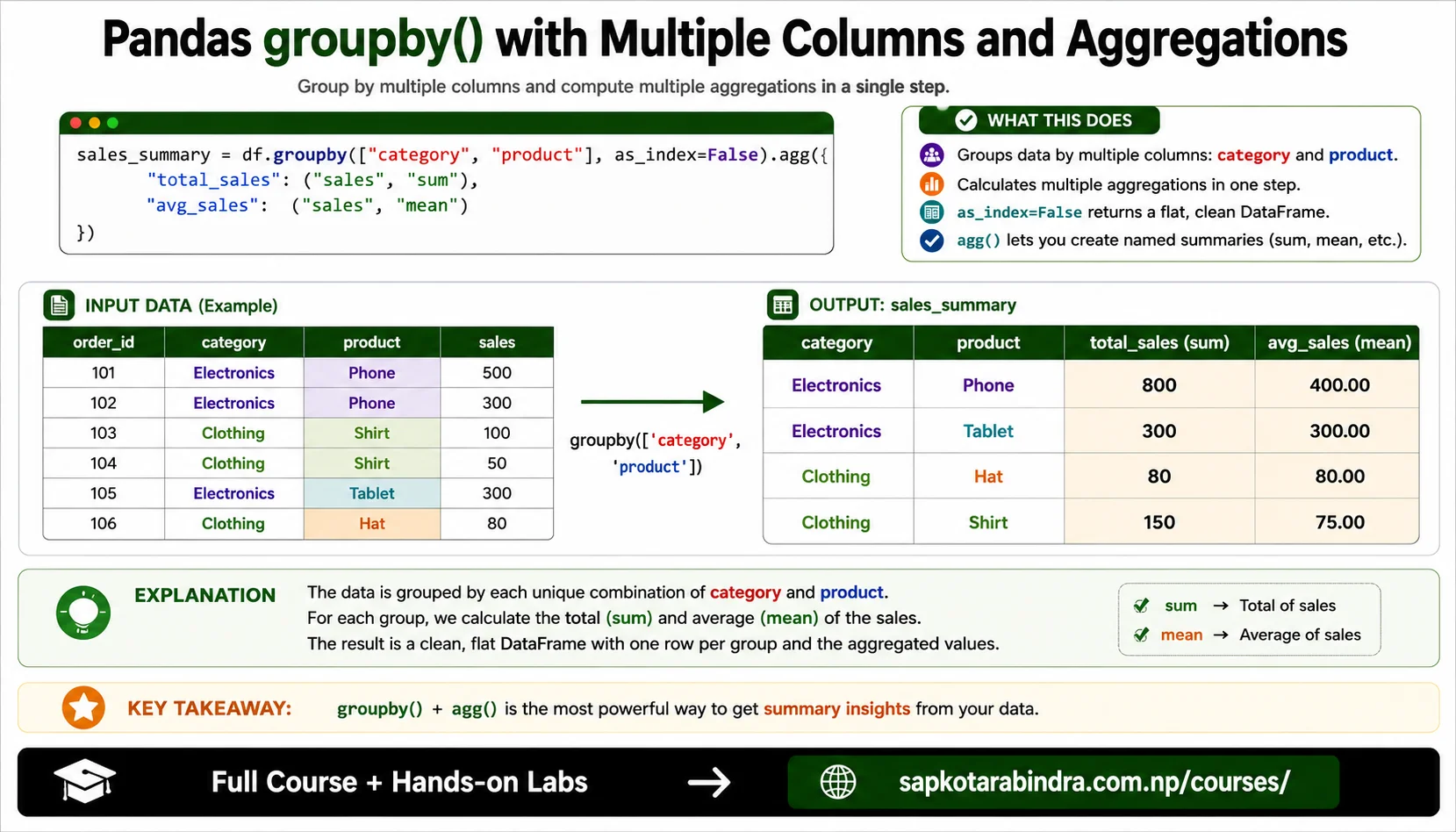
groupby()is used to group data and calculate summary values. Example: Find total sales for each category.- Common functions include: 👉 sum 👉 mean 👉 count 👉 min 👉 max 👉 std 👉 median 👉 quantile 👉 idxmin 👉 idxmax 👉 unique 👉 nunique 👉 cumsum 👉 prod 👉 mode 👉 var
total_sales = df["sales"].sum()print(total_sales)sales_summary = df.groupby(["category", "product"],as_index=False).agg(total_sales=("sales", "sum"),avg_sales=("sales", "mean"))print(sales_summary)📌 Simple idea:groupby()creates groups.agg()calculates summary values for each group.
11.1 📊 What is GroupBy?
11.2 Common Aggregation Functions
11.3 Basic Aggregation
11.4 GroupBy Example
12. Time Series Operations
- Time series data is data that changes over time. Examples: - Daily sales - Monthly revenue - Hourly temperature - Stock prices Pandas has powerful tools for working with time-based data.
- Before doing time series operations, convert the date column to datetime.
df["date"] = pd.to_datetime(df["date"]) - For resampling, the index usually needs to be datetime.
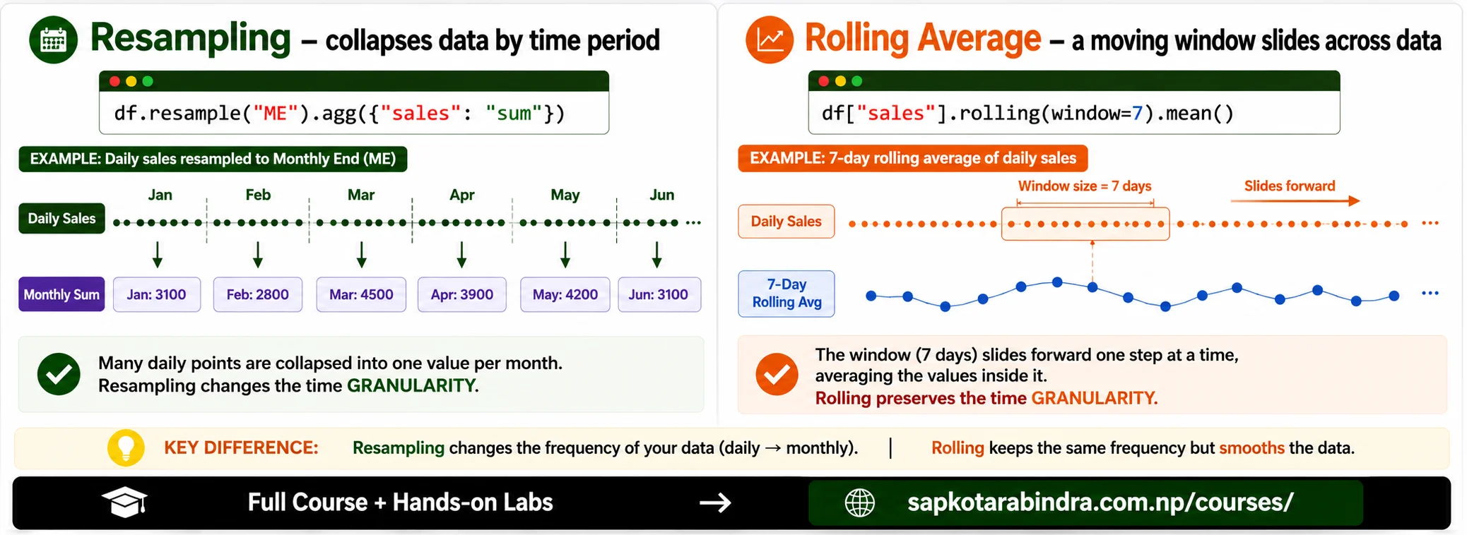
df.set_index("date", inplace=True) - Resampling means changing the frequency of time-based data.
12.1 🕒 What is Time Series Data?
12.2 Convert Date Column to Datetime
12.3 Set Date as Index
12.4 Resampling
Common Frequency Codes
| Code | Meaning |
|---|---|
| D | Daily |
| W | Weekly |
| MS | Month start |
| ME | Month end |
| QS | Quarter start |
| QE | Quarter end |
| YS | Year start |
| YE | Year end |
monthly_sales = df.resample("ME").agg({"sales": "sum"})- Rolling average calculates the average over a moving window.
df["rolling_avg"] = df["sales"].rolling(window=7).mean()📌 Simple idea: Resampling summarizes data by time period. Rolling calculates moving values.
12.5 Monthly Sales Example
12.6 Rolling Average
13. String and Datetime Functions
- String functions are applied to text columns using
.str.df["name"] = df["name"].str.upper()df["name"] = df["name"].str.strip()df["name"] = df["name"].str.replace("old", "new") - Datetime functions are applied to datetime columns using
.dt.df["year"] = df["date"].dt.yeardf["day"] = df["date"].dt.daydf["day_of_week"] = df["date"].dt.day_name()📌 Simple idea: Use.strfor text columns. Use.dtfor datetime columns.
13.1 🔤 String Functions with .str
13.2 Datetime Functions with .dt