
Pandas: Loading Data & EDA
✕1. Introduction to Pandas
- Pandas is a Python library used for: 👉 Loading data 👉 Analyzing data 👉 Transforming data 👉 Cleaning data 👉 Saving processed data 📌 Imagine trying to filter, sort, and summarize a spreadsheet using only Python lists. Pandas gives us spreadsheet-like power directly inside Python. Pandas is very useful in Data Science because most real-world data comes in table-like format. Examples: - CSV files - Excel files - SQL tables - JSON files - Python lists or dictionaries
- Pandas is an external library, so we need to install it first.
Installation Code:
pip install pandasThen we import it in Python:import pandas as pd📌pdis the common short name used for Pandas. - A DataFrame is the main data structure in Pandas. It is a 2D labelled data structure, similar to a table.
1.1 🐼 What is Pandas?
1.2 Installing Pandas
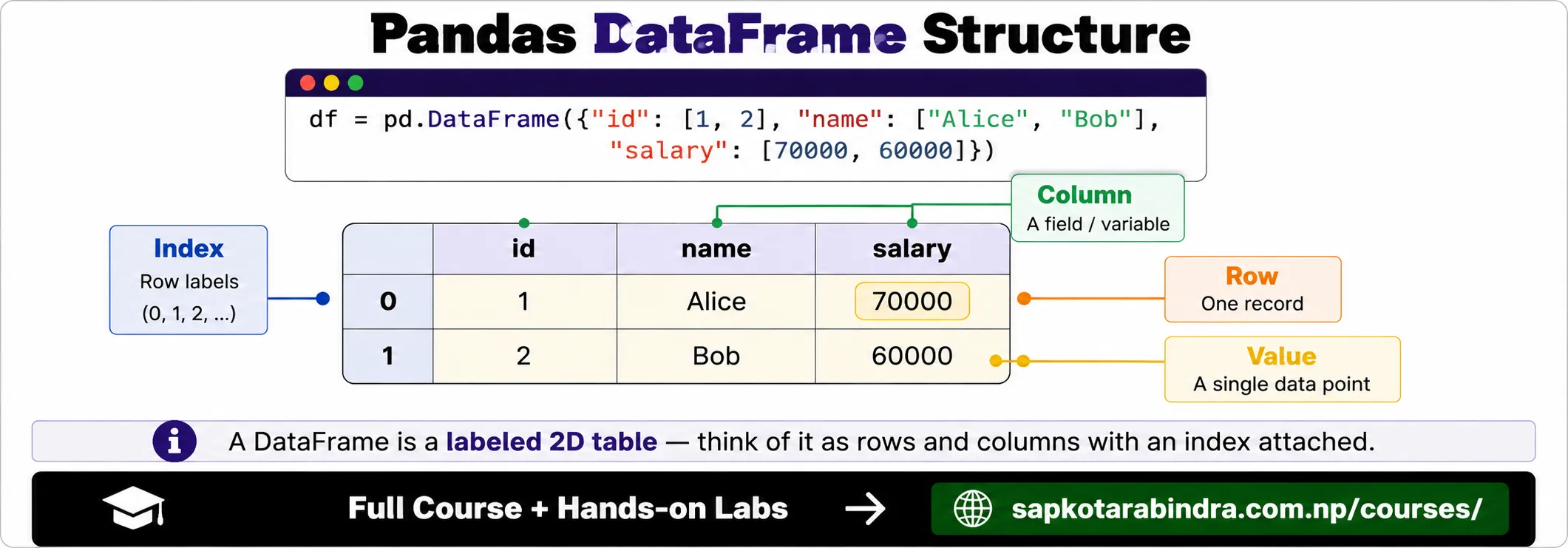
1.3 What is a DataFrame?
| id | name | salary |
|---|---|---|
| 1 | Alice | 70000 |
| 2 | Bob | 60000 |
- A DataFrame has: - Rows - Columns - Index - Values 📌 A DataFrame is like an Excel sheet or SQL table inside Python.
1.3.1 Note
- With Pandas, we can perform operations like: ✅ Selecting columns ✅ Filtering rows ✅ Sorting data ✅ Grouping data ✅ Joining tables ✅ Handling missing values ✅ Reading and writing files 📌 Pandas helps us work with tabular data easily.
1.4 Why Use Pandas?
2. Loading CSV with Pandas
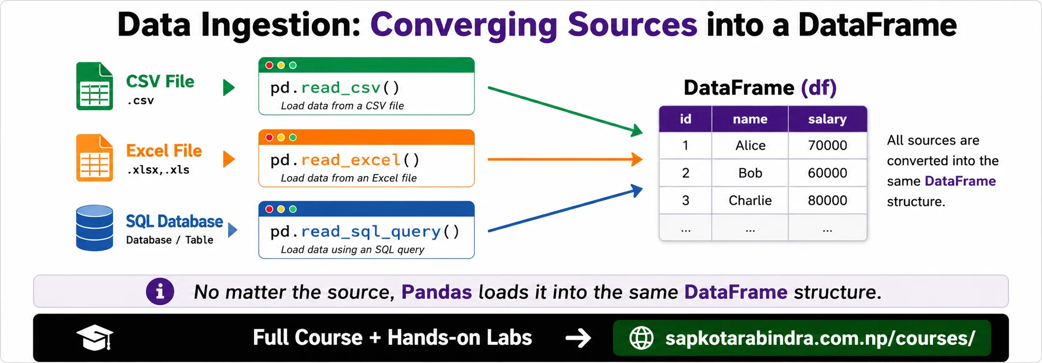
- A CSV file can be loaded into a DataFrame using
pd.read_csv(). import pandas as pd# Load CSV file into DataFramefile_path = r"folder_1/folder_2/file.csv"df = pd.read_csv(file_path)# Display first few rowsprint(df.head())# Display last 2 rowsprint(df.tail(2))# Display random 5 rowsprint(df.sample(5))# Display column namesprint(df.columns)📌pd.read_csv()reads a CSV file and converts it into a DataFrame.
2.1 📄 Loading a CSV File
2.2 Example: Load CSV
3. Common Arguments of pd.read_csv()
pd.read_csv()accepts different arguments to control how the file is loaded.
3.1 Why Use Arguments?
3.2 Common Arguments
| Argument | Description | Example |
|---|---|---|
sep | Delimiter used to separate values. Default is comma | pd.read_csv("file.csv", sep="\t") |
nrows | Number of rows to read | pd.read_csv("file.csv", nrows=100) |
skiprows | Number of rows to skip from the top | pd.read_csv("file.csv", skiprows=5) |
header | Row number to use as column names | pd.read_csv("file.csv", header=0) |
names | Custom column names | pd.read_csv("file.csv", names=["col1", "col2"]) |
usecols | Select only specific columns | pd.read_csv("file.csv", usecols=["col1", "col2"]) |
encoding | Encoding of the file | pd.read_csv("file.csv", encoding="utf-8") |
import pandas as pddf = pd.read_csv("file.csv", usecols=["name", "salary"])print(df.head())📌 Simple idea: Arguments help us load only the data we need.
3.3 Example: Read Only Selected Columns
4. Loading Excel with Pandas
- Excel files can be loaded into a DataFrame using
pd.read_excel(). To read .xlsx files, we usually need theopenpyxllibrary. Install it using:pip install openpyxl import pandas as pd# Load first sheetdf = pd.read_excel(r"folder_1/folder_2/file.xlsx")print(df.head())df = pd.read_excel(r"folder_1/folder_2/file.xlsx", sheet_name="s_1")print(df.head())
4.1 📘 Loading Excel Files
4.2 Example: Load Excel File
4.3 Load Specific Sheet
5. 🗄️ Loading Data from SQL with Pandas
- Pandas can read data from SQL databases using
pd.read_sql_query(). To connect to databases, we usually use SQLAlchemy. Install it using:pip install sqlalchemyFor PostgreSQL, we may also need:pip install psycopg2-binary - General format:
dialect+driver://username:password@host:port/databaseExample for PostgreSQL:postgresql+psycopg2://username:password@host:port/database import pandas as pdfrom sqlalchemy import create_engineconnection_string = "postgresql+psycopg2://username:password@localhost:5432/database_name"engine = create_engine(connection_string)# Engine manages the connection between Pandas and the databasedf = pd.read_sql_query("SELECT * FROM table_name", engine)print(df.head())engine.dispose()📌 Pandas can read SQL query results directly into a DataFrame.
5.1 Reading SQL Data
5.2 Connection String Format
5.3 Example: Read SQL Table
6. 🔌 Common Connection Strings
| Database | Connection String Format |
|---|---|
| SQLite | sqlite:///path_to_db.db |
| PostgreSQL | postgresql+psycopg2://username:password@host:port/database |
| MySQL | mysql+pymysql://username:password@host:port/database |
| SQL Server | mssql+pyodbc://username:password@host:port/database?driver=ODBC+Driver+17+for+SQL+Server |
| Oracle | oracle+cx_oracle://username:password@host:port/database |
7. 🧱 Creating DataFrame from Python Data
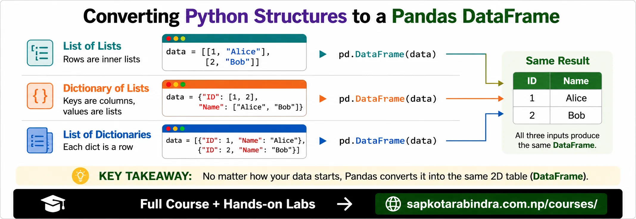
- A DataFrame can also be created from Python data structures like: ✅ List ✅ Dictionary ✅ List of dictionaries
import pandas as pddata = [[1, "Alice"],[2, "Bob"],[3, "Charlie"]]df = pd.DataFrame(data, columns=["ID", "Name"])print(df)import pandas as pddata = {"ID": [1, 2, 3], "Name": ["Alice", "Bob", "Charlie"]}df = pd.DataFrame(data)print(df)import pandas as pddata = [{"ID": 1, "Name": "Alice"},{"ID": 2, "Name": "Bob"}]df = pd.DataFrame(data)print(df)
7.1 🧱 Creating DataFrames Manually
7.2 From List
7.3 From Dictionary
7.4 From List of Dictionaries
8. 🔍 Exploratory Data Analysis with Pandas
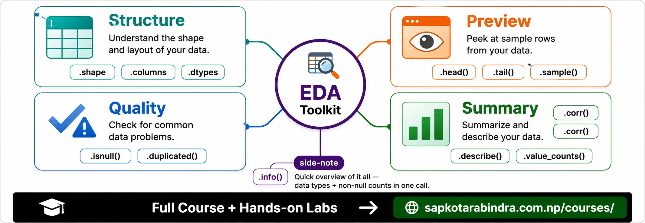
- EDA means Exploratory Data Analysis. It is the process of understanding the main characteristics of data. During EDA, we usually check: ✅ Number of rows and columns ✅ Column names ✅ Data types ✅ Missing values ✅ Duplicate values ✅ Summary statistics ✅ Unique value counts ✅ Correlations
8.1 What is EDA?
8.2 Common Pandas Functions for EDA
| Function | Description | Example |
|---|---|---|
.shape | Returns number of rows and columns | df.shape |
.head() | Returns first n rows | df.head(5) |
.tail() | Returns last n rows | df.tail(2) |
.sample() | Returns random n rows | df.sample(4) |
.columns | Returns column labels | df.columns |
.dtypes | Returns data types of columns | df.dtypes |
.info() | Shows summary including data types and non-null counts | df.info() |
.describe() | Generates summary statistics | df.describe() |
.value_counts() | Counts unique values in a column | df["column"].value_counts() |
.isnull() | Detects missing values | df.isnull().sum() |
.duplicated() | Detects duplicate rows | df.duplicated().sum() |
.corr() | Computes correlation of numeric columns | df.corr(numeric_only=True) |
import pandas as pddf = pd.read_csv("file.csv")print(df.shape)print(df.head())df.info()print(df.describe())print(df.isnull().sum())print(df.duplicated().sum())📌 EDA helps us understand data before cleaning or modeling.
8.3 Example: Basic EDA
9. 📊 Data Profiling Report using ydata-profiling
ydata-profilingis an external library used to generate a detailed data profiling report. It creates an interactive HTML report with details about: 👉 Data quality 👉 Missing values 👉 Distributions 👉 Correlations 👉 Possible data issues Install it using:pip install ydata-profilingimport pandas as pdfrom ydata_profiling import ProfileReportdf = pd.read_csv(r"path_to_your_data.csv")profile = ProfileReport(df, title="Data Profiling Report")profile.to_file("report.html")📌 Note:ydata-profilingcan sometimes have compatibility issues with newer Python versions.
9.1 What is ydata-profiling?
9.2 Example: Generate Profiling Report
10. Pandas Series
- A Series is a one-dimensional labelled array in Pandas. A single column from a DataFrame is usually a Series.
Example:
age_series = df["age"]📌 DataFrame is like a full table. Series is like one column.
10.1 📌 What is a Series?
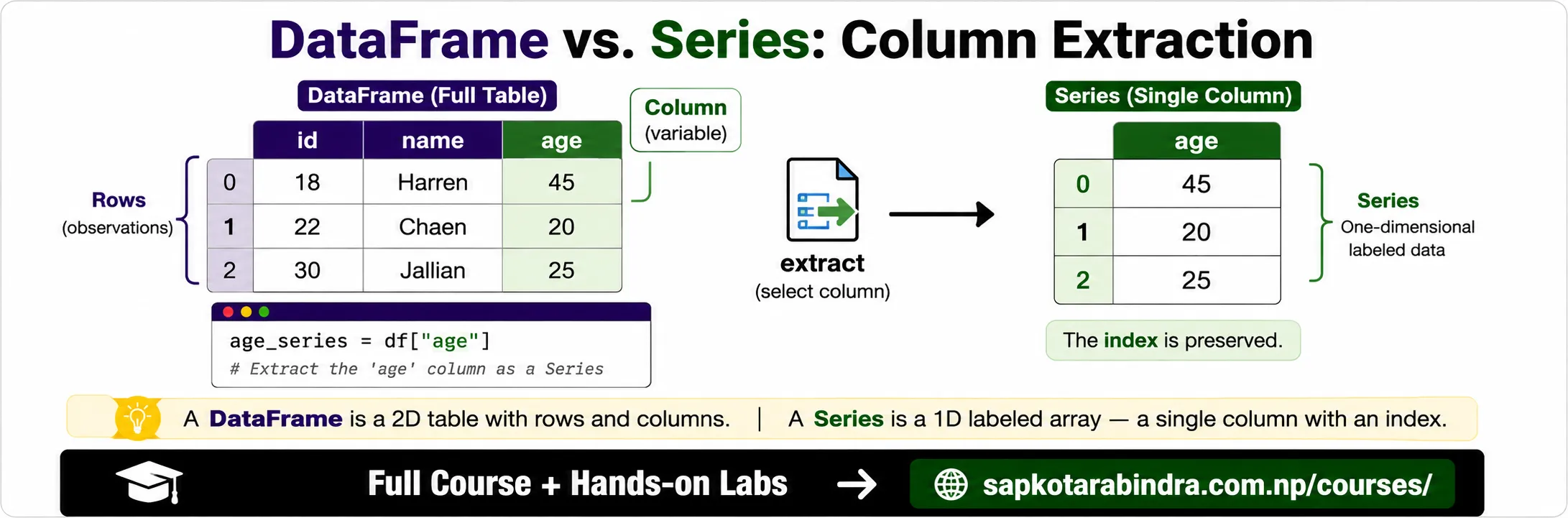
import pandas as pddf = pd.read_csv(r"base_ball_data_path.csv")age_series = df["age"]filtered_age = age_series[age_series < 22]print(filtered_age)print(filtered_age.mean())- Pandas Series supports element-wise operations, similar to NumPy.
bmi_series = df["weight"] / (df["height"] ** 2)print(bmi_series + 1)📌 Operations on a Series are applied value by value.
10.2 Series Example
10.3 Element-wise Operations
11. 💾 Writing DataFrame to File or Database
- After filtering, cleaning, or transforming data, we often need to save the result. A DataFrame can be saved to: ✅ CSV ✅ Excel ✅ SQL database
df.to_csv("filtered_data.csv", index=False)This saves the DataFrame as a CSV file without writing the index column.df.to_csv("filtered_pipe.psv", sep="|", index=False)df.to_excel("data.xlsx", index=False)df.to_sql("table_name", engine, if_exists="replace", index=False)
11.1 💾 Why Save Data?
11.2 Save DataFrame to CSV
11.3 Save DataFrame as Pipe-Separated File
11.4 Save DataFrame to Excel
11.5 Save DataFrame to SQL
Common values for if_exists
| Value | Meaning |
|---|---|
| fail | Fails if table already exists |
| replace | Drops old table and creates new one |
| append | Adds data to existing table |
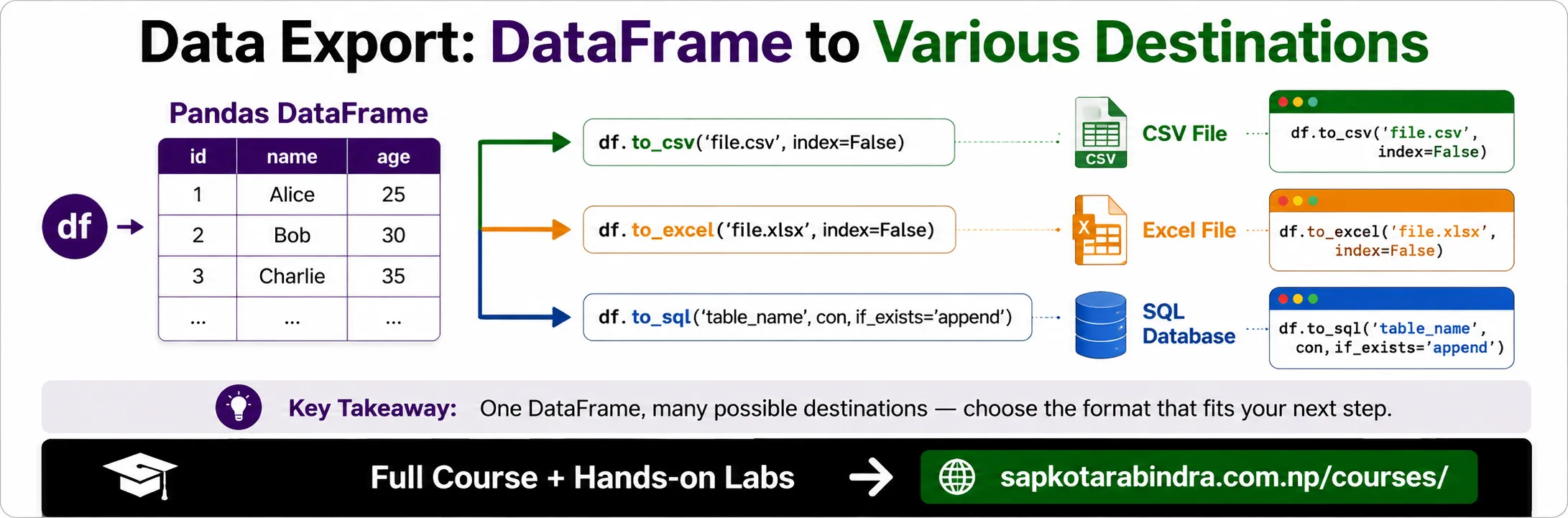
- 📌 Simple idea: Use
to_csv(),to_excel(), orto_sql()depending on where you want to save the DataFrame.
11.6 Note