
Descriptive Statistics
✕Variable
- A characteristic or attribute that can take on different values.
- Basic unit of analysis in statistics and data science.
- Example: In customers data, variables might include
age,gender,income,expenditure. - Numerical (Quantitative): Represent measurable quantities. Further divided as: - Discrete: Countable values (e.g., number of customers). - Continuous: Any value within a range (e.g., height, weight).
- Categorical (Qualitative): Represent categories or groups. Further divided as: - Nominal: No inherent order (e.g., gender, color). - Ordinal: Inherent order (e.g., customer review, T-Shirt size).
Types of Variables
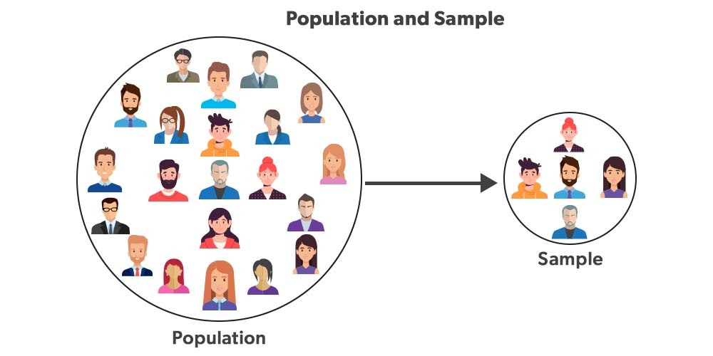
Sample VS Population
- Population: The entire group of instances about whom we hope to learn.
- Sample: A subset from population that is used to in statistical analysis.
- We use samples as it is often impractical to collect data from an entire population.
- Example:
- Selecting random
1000people from population of1 millionto estimate income. - Using a sample of500reviews to estimate average customer satisfaction score. - Key point: Sample should be representative of the population to make valid inferences. This is often achieved through random sampling techniques.
- Sampling bias can lead to inaccurate conclusions if the sample is not representative of the population. We will use stratified sampling in ML models to avoid bias.
Statistics
- Science of collecting, analyzing, interpreting, and presenting data.
- Descriptive Statistics: Summarizes & describes the main features of a dataset (e.g.,
mean,median,mode,standard deviationetc.). - Inferential Statistics: Makes predictions or inferences about a population based on a sample of data (e.g.,
hypothesis testing,confidence intervals). - Used in data science to understand data distributions, relationships, and to make informed decisions based on data.
- Example: A data scientist might use descriptive statistics to summarize customer purchase behavior and inferential statistics to determine if a new marketing strategy has significantly increased sales.
Types:
Central Tendency
- Measures that represent the center / typical value of a data. Common Measures :
- Arithmetic average of a set of values. i.e
mean(X̄) = Σx / N. - Takes into account all values, making it sensitive to outliers.
- For
[2, 1, 2, 5, 100], X̄ =(2 + 1 + 2 + 5 + 100)/5 = 110 / 5 = 22, false representative. - Single in single data point changes the mean drastically.
- Best used for numerical data having symmetrical distributions without outliers.
- Middle value when data is sorted.
- If even number of values, it is the average of the two middle values.
- Calculated on basis of position, not magnitude, making it robust to outliers.
- For
[2, 1, 2, 5, 100], median =2, a much better representative of the typical value. - Best used for numerical data with skewed distributions or outliers.
- Most frequently occurring value(s) in a dataset.
- Can be used for both numerical and categorical data.
- For
[2, 1, 2, 5, 100], mode =2.
Mean
Median
Mode
Percentiles and Quartiles
- Give information about the position of a value relative to the rest of the data.
- Single mean is incomplete summary unless we know how data is distributed around it.
- We can't consider score 60 / 100 as good or bad without knowing how other scored.
- Values that divide a dataset into 100 equal parts.
- The
p-th percentile is the value below whichp%of the data falls. - Example: Student scores in the 90th => They scored better than 90% of the other.
- Values that divide a dataset into 4 equal parts.
- The
Q1(25th percentile) is the value below which 25% of the data falls. - The
Q2= 50th percentile is the median. - The
Q3(75th percentile) is the value below which 75% of the data falls. - The inter-quartile range (IQR) is the difference between Q3 and Q1
IQRis a measure of variability that is robust to outliers.- Data below
Q1 - 1.5 * IQRand aboveQ3 + 1.5 * IQRare considered outliers.
Percentiles
Quartiles
Dispersion
- Measures that represent the spread or variability of data. Common Measures :
- Difference between the maximum and minimum values in a dataset.
- Highly sensitive to outliers.
- Best used for quick, rough estimate of variability but not for detailed analysis.
- Formula:
Range = Max - Min. For[2, 1, 2, 5, 100], range =100 - 1 = 99 - Average of the squared differences from the mean.
- High Variance => data points are spread out from the mean
- Low Variance => data points are close to the mean.
- Formula:
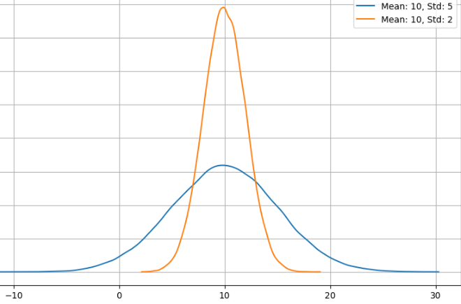
Variance = Σ(Xi - X̄)² / N. [5, 20, 95]and[38, 40, 42]have same mean40but variance1550and2.67.- Square root of the variance. i.e
Std Dev = sqrt(Variance). - Expressed in the same units as the data, making it more interpretable than variance.
- For
[5, 20, 95], std dev =39.37and for[38, 40, 42], std dev =1.63.
Range / Peak To Peak
Variance
Standard Deviation
Normal Distribution for Same Mean, Different Variance
Example of Dispersion Calculation
- For data points
[5, 20, 95]: - Mean =
(5 + 20 + 95)/ 3 = 40, Min =5, Max =95, Range =Max - Min = 95 - 5 = 90
Calculation of Variance and Standard Deviation:
| Value (X) | Difference from Mean (X - X̄) | Squared Difference i.e. (X - X̄)² |
|---|---|---|
| 5 | 5 - 40 = -35 | (-35)² = 1225 |
| 20 | 20 - 40 = -20 | (-20)² = 400 |
| 95 | 95 - 40 = 55 | (55)² = 3025 |
| Variance | (1225 + 400 + 3025) / 3 = 1550 | |
| Standard Deviation | sqrt(1550) = 39.37 |
Example showing calculation of Variance and Standard Deviation
Covariance and Correlation
- Measure of how two variables change together.
- Positive covariance => both variables
increase or decrease together. - Negative covariance => one variable increases while the other decreases.
- Zero covariance => no relationship between variables.
- Does not indicate strength of relationship and is sensitive to scale.
- Formula:
Cov(X,Y) = Σ((Xi - X̄) * (Yi - Ȳ)) / n# n -1 for sample. - Did you Notice:
COV(X, X) = Σ((Xi - X̄) * (Xi - X̄)) / n = Σ(Xi - X̄)² / n = Var(X) - Standardized measure of strength & direction of relationship between two variables.
- Formula:
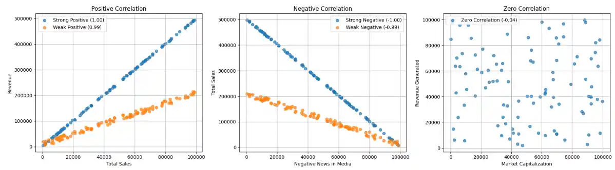
Correlation = Cov(X,Y) / (Std Dev X * Std Dev Y) - Value of correlation always lies between -1 to 1.
1=> strong positive,-1=> strong negative,0=> weak or no relationship.- Correlation is unitless and allows comparison across different variable pairs.
Covariance
Correlation
Plot showing different types of correlation
Example: Covariance, Correlation Calculation
- For data points X =
[5, 20, 95]and Y =[10, 30, 50]: - X̄ =
(5 + 20 + 95)/ 3 = 40, Ȳ =(10 + 30 + 50) / 3 = 30
Calculation of Covariance and Correlation:
| X | X - X̄ | (X - X̄)² | Y | Y - Ȳ | (Y - Ȳ)² | (X - X̄) * (Y - Ȳ) |
|---|---|---|---|---|---|---|
| 5 | 5 - 40 = -35 | (-35)² = 1225 | 10 | 10 - 30 = -20 | 400 | (-35) * (-20) = 700 |
| 20 | 20 - 40 = -20 | (-20)² = 400 | 30 | 30 - 30 = 0 | 0 | (-20) * (0) = 0 |
| 95 | 95 - 40 = 55 | 55² = 3025 | 50 | 50 - 30 = 20 | 400 | 55 * 20 = 1100 |
| Var(X) | (1225+400+3025)/ 3 = 4650 | Var(Y) | (400+0+400)/3 = 266.67 | COV =(700+0+1100)/3 = 600 | ||
| Std(X) | sqrt(4650) = 68.18 | Std(Y) | sqrt(266.67) = 16.33 | Corr = 600 / (68.18 * 16.33) = 0.54 |
Example showing calculation of Covariance and Correlation
Spearman Rank Correlation
- Used to find correlation when data is ordinal or not normally distributed.
- Ranks data points and computes correlation on ranks rather than raw values.
- Formula:
ρ = 1 - (6 * Σd²) / (n * (n² - 1)),d=> rank difference for each pair. - For data:
t_shirt = ['M', 'S', 'L', 'XL'],customer_satisfaction = [3, 4, 2, 5].
Spearman Rank Correlation for T-shirt size and Satisfaction
| T-shirt Size | Rank T-shirt (R1) | Customer Satisfaction | Rank Satisfaction (R2) | d = R1 - R2 | d² |
|---|---|---|---|---|---|
| M | 2 | 3 | 2 | 2 - 2 = 0 | 0² = 0 |
| S | 1 | 4 | 3 | 1 - 3 = -2 | -2² = 4 |
| L | 3 | 2 | 1 | 3 - 1 = 2 | 2² = 4 |
| XL | 4 | 5 | 4 | 4 - 4 = 0 | 0² = 0 |
| n = 4 | n(n²-1) = 4(4²-1) = 60 | Σd² = 8 | ρ = 1-6*8/60 =0.2 |
Ranking and calculation of Spearman correlation
Probability
- Measure of the likelihood that an event will occur.
- It ranges from 0 to 1, where 0 => certainly not occur and 1 => certainly occur.
- Used in data science to make predictions and decisions based on uncertain data.
- Example: If a model predicts a 0.8 probability of rain tomorrow, it means there's an 80% chance of rain, and you might decide to carry an umbrella.
- Probability is calculated as:
P(A) = Number of favorable outcomes / Total number of outcomes. - Rule:
P(A)+P(not A)=1,P(A or B)=P(A)+P(B)-P(A and B),P(A and B)=P(A)*P(B|A)=P(B)*P(A|B). - Suppose you have a deck of 52 cards: - If you draw one card. What is it's probability being face card? - If you draw one card. What is it's probability being ace or heart? - If you draw two cards, what is probability both being face card?
Bayes Theorem Practical Example
- Lionel Messi played
578games (294home &284away) for barcelona. He scored38hatricks at home and20hatricks away. If he scored a hatrick, what is the probability that it was at home? - Let
H => Home Game,A => Away Game,T => Hatrick. We need to calculateP(H|T). P(H) = 294 / 578 = 0.51,P(A) = 284 / 578 = 0.49P(T|H) = 38 / 294 = 0.13,P(T|A) = 20 / 284 = 0.07.P(T) = P(T|H) * P(H) + P(T|A) * P(A) = 0.13 * 0.51 + 0.07 * 0.49 = 0.10- Now:
P(H|T) * P(T) = P(T|H) * P(H)P(H|T) * 0.10 = 0.13 * 0.51P(H|T) = (0.13 * 0.51) / 0.10 = 0.66 - Interpretation that if Messi scored a hatrick, there is a 66% chance it was at home.