
Support Vector Machines
✕SVM Concept
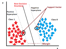
- Find the hyperplane that best separates classes with maximum margin.
- Support vectors: Data points closest to the hyperplane.
- Margin: Distance between the hyperplane and support vectors.
- Maximizing margin leads to better generalization on unseen data.
SVM Algorithm Steps
- Identify the Support Vectors.
- Find Hyperplane
ax + by + c = 0, such that it will have maximum distance from Support Vectors. - During prediction, evaluate a point with hyperplane equation
ax1 + by1 + c. - Assign Label according to the sign of the result.
Sample Data for SVM
SVM Example with Two Classes:
| Point | Feature A | Feature B | Class |
|---|---|---|---|
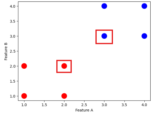
| P1 | 1 | 2 | Red |
| P2 | 2 | 1 | Red |
| P3 | 3 | 4 | Blue |
| P4 | 4 | 3 | Blue |
| P5 | 1 | 1 | Red |
| P6 | 2 | 2 | Red |
| P7 | 3 | 3 | Blue |
| P8 | 4 | 4 | Blue |
Dataset for SVM example with two classes.
SVM Alogrithm Visually: Step 1
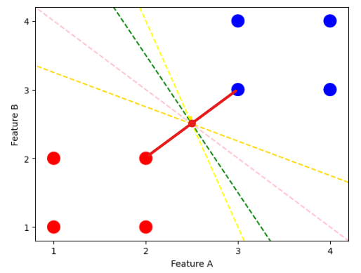
SVM Algorithm Visually: Step 2
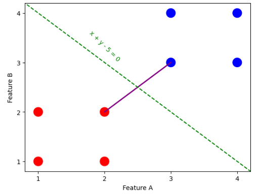
SVM Algorithm Visually: Step 3
SVM Algorithm Mathematically
Distance Calculation for SVM:
| P3: (3, 4) | P4: (4, 3) | P7: (3, 3) | P8: (4, 4) | |
| P1: (1, 2) | √((3-1)² + (4-2)²) = 2.83 | √((4-1)² + (3-2)²) = 2.24 | √((3-1)² + (3-2)²) = 2.24 | √((4-1)² + (4-2)²) = 3.16 |
| P2: (2, 1) | √((3-2)² + (4-1)²) = 3.16 | √((4-2)² + (3-1)²) = 2.83 | √((3-2)² + (3-1)²) = 2.24 | √((4-2)² + (4-1)²) = 2.83 |
| P5: (1, 1) | √((3-1)² + (4-1)²) = 3.61 | √((4-1)² + (3-1)²) = 3.16 | √((3-1)² + (3-1)²) = 2.83 | √((4-1)² + (4-1)²) = 4.24 |
| P6: (2, 2) | √((3-2)² + (4-2)²) = 2.24 | √((4-2)² + (3-2)²) = 2.24 | √((3-2)² + (3-2)²) = 1.41 | √((4-2)² + (4-2)²) = 2.83 |
Distance calculation from support vectors to the hyperplane in SVM.
Calculating Hyperplane for SVM:
Support Vectors: P6 (Red): (2, 2), P7 (Blue): (3, 3) |
Midpoint: (2+3)/2, (2+3)/2 = (2.5, 2.5) |
Slope of Line Connecting Support Vectors: m = (3-2)/(3-2) = 1 |
Slope of Hyperplane: m_hyperplane = -1/m = -1 |
Equation of Hyperplane: y - 2.5 = -1(x - 2.5) => y - 2.5 = -x + 2.5 => x + y - 5 = 0 |
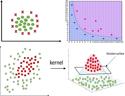
Kernel Trick for Non-Linear SVM
- SVM can be extended to non-linear decision boundaries using kernel functions.
- Kernel functions implicitly map input features into higher-dimensional space where linear separation is possible.
- Common Kernels: Linear, Polynomial, Radial Basis Function (RBF), Sigmoid.
- RBF kernel is popular for non-linear problems as it can capture complex relationships.
SVM Hyperparameters
SVM Hyperparameters and their Effects:
| Hyperparameter | Description | Effect on Model |
|---|---|---|
| C: Regularization Parameter | Controls trade-off between maximizing margin and minimizing classification error. | Small C => wider margin but more misclassifications (underfitting), Large C => narrower margin but fewer misclassifications (overfitting). |
| kernel: Kernel Type | Specifies the kernel function to use (e.g. linear, rbf, poly). | Different kernels can capture different types of relationships in the data. |
| gamma: Kernel Coefficient | Defines how far the influence of a single training example reaches (only for RBF, Poly, Sigmoid). | Small gamma => far reach (smooth decision boundary), Large gamma => close reach (more complex decision boundary). |
degree: Degree of the polynomial kernel function (only for poly kernel). | Higher degree allows for more complex decision boundaries but can lead to overfitting. | Small degree => simpler decision boundary, Large degree => more complex decision boundary. |
Key hyperparameters for SVM and their impact on model performance.