
Descriptive Statistics
✕1. Variable
- A variable is a piece of information that can have different values. In simple words:
A variable is something we can measure, record, or observe.
If we collect data about customers, each customer may have different values for:
age,gender,income,expenditure,city,number_of_ordersEach of these is called a variable. - Variables are mainly divided into two types: - Numerical Variables - Categorical Variables
1.1 📦 What is a Variable?
1.2 🔢 Types of Variables
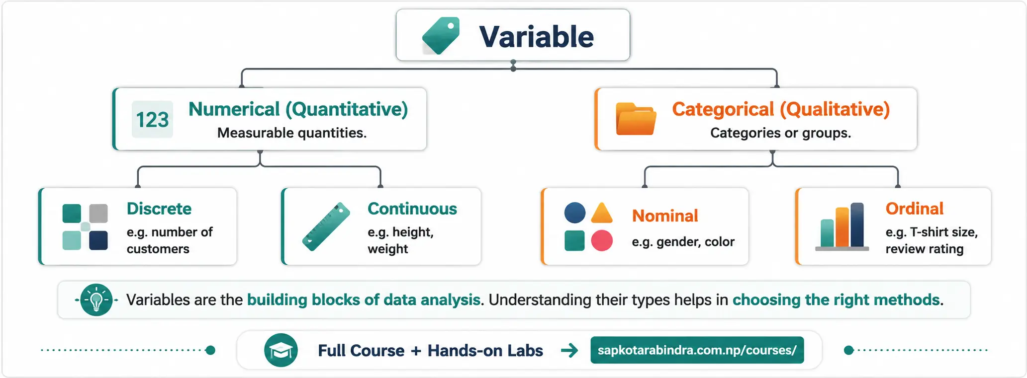
Numerical Variables
| Type | Description | Example |
|---|---|---|
| Continuous 📏 | Measurable value; can include decimals | Height, Weight, Temperature |
| Discrete 🔢 | Countable values, usually whole numbers | Total Books, Number of Cars, Order Count |
Types of Numerical Variables
Categorical Variables
| Type | Description | Example |
|---|---|---|
| Nominal 🏷️ | Categories with no meaningful order. | Colors, Gender, Blood Group |
| Ordinal 📶 | Categories with meaningful order. | Education Level, Rating |
Types of Categorical Variables
2. Population vs Sample
- A population is the entire group we want to study. Examples: - All students in a school - All customers of a company - All people living in a city - All products sold by a shop
- A sample is a smaller group selected from the population. We study the sample to understand the larger population. If a city has 1 million people, it may be difficult to ask everyone about their income. So, we may randomly select 1,000 people and study them. Here: Population = 1 million people Sample = 1,000 selected people
- We use samples because studying the entire population can be: - Too expensive 💰 - Too time-consuming ⏰ - Difficult to manage 📋 - Sometimes impossible 😵 So, we study a smaller group and use it to make conclusions about the larger group.
- A sample should fairly represent the population, meaning it should give a balanced picture of the whole group. If we want to know the opinion of all students in a school, we should not ask only Grade 10 students. We should include students from different grades. 📌 A good sample gives a fair picture of the whole population.
2.1 🌍 What is Population?
2.2 👥 What is Sample?
2.3 🤔 Why Do We Use Samples?
2.4 🎯 Representative Sample
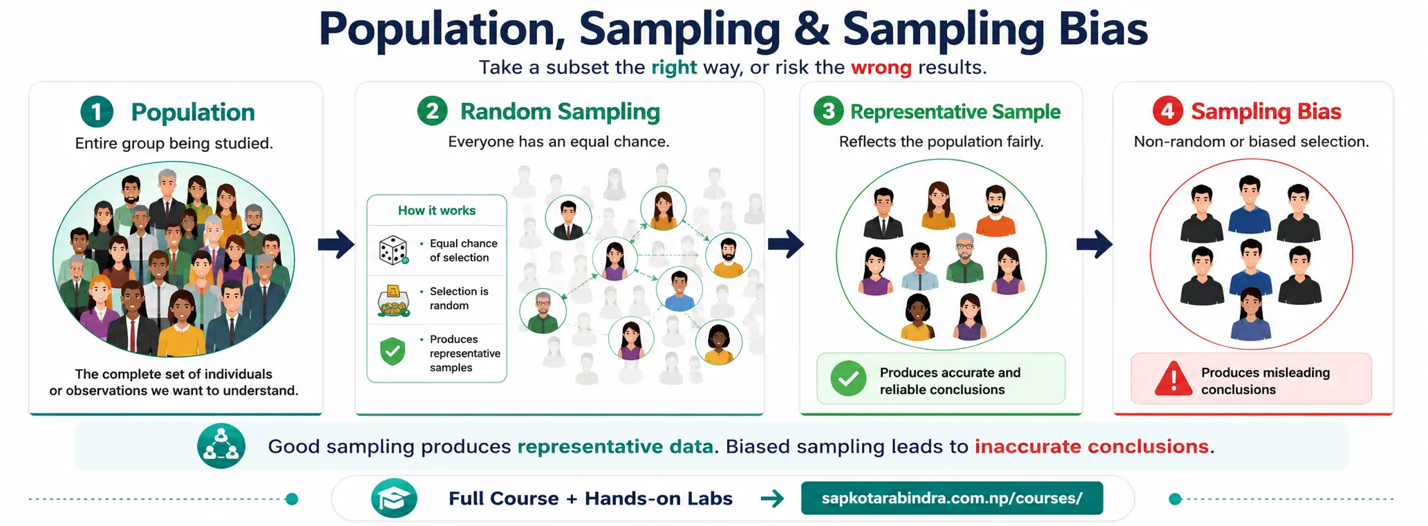
- Sampling bias happens when the sample does not properly represent the population. If we ask only cricket fans about their favorite sport, most may say cricket. But that does not mean everyone likes cricket the most. 📌 A biased sample can lead to wrong conclusions.
2.5 ⚠️ Sampling Bias
3. Statistics
- Statistics is the science of: ✅ Collecting data ✅ Organizing data ✅ Analyzing data ✅ Understanding data ✅ Presenting data clearly In simple words: Statistics helps us make sense of data.
- There are two main types of statistics: - Descriptive Statistics - Inferential Statistics
3.1 📊 What is Statistics?
3.2 📋 Types of Statistics
Types of Statistics
| Type | Description | Example |
|---|---|---|
| Descriptive Statistics 📉 | Summarizes and describes existing data. | Mean, Median, Mode, Standard Deviation |
| Inferential Statistics 🔮 | Uses sample data to make conclusions about a larger group | Hypothesis testing, Confidence intervals, Prediction from sample data |
Types and Examples of Statistics
4. Central Tendency
- Central tendency tells us the center or typical value of data. It helps answer: What value represents this data best? The three most common measures are: - Mean - Median - Mode
- Mean is the arithmetic average of numbers.
Formula:
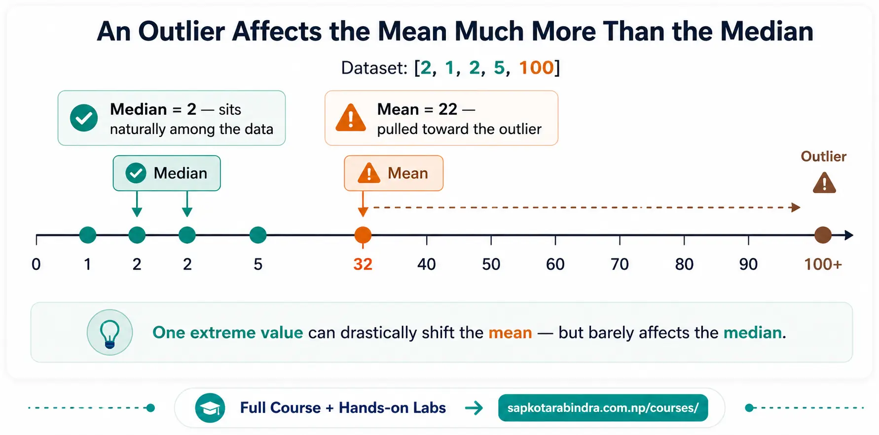
Mean = Sum of all values / Number of valuesFor data:[2, 1, 2, 5, 100],mean = (2 + 1 + 2 + 5 + 100) / 5 = 22⚠️ Mean can be affected by very large or very small values called outliers. 📌 In this example, 100 makes the mean much larger than most values. - Median is the middle value after sorting the data.
Steps:
1. Sort the data
2. Find the middle value
Example:
Original data:
[2, 1, 2, 5, 100]Sorted data:[1, 2, 2, 5, 100]Middle value:2So, the median is2. ✅ Median is useful when data has outliers. 📌 Here, median 2 represents the data better than mean 22.
4.1 🎯 What is Central Tendency?
4.2 ➗ Mean
4.3 📍 Median
- Mode is the value that appears most often.
Example:
For data:
[2, 1, 2, 5, 100]The value 2 appears most often, so the mode is 2.data = ["Red", "Blue", "Red", "Green", "Red"]Mode isRedbecause it appears most often. Mode works for both numerical and categorical data.
4.4 🔁 Mode
4.5 🧠 When to Use Mean, Median, and Mode
| Measure | Best Used When |
|---|---|
| Mean ➗ | Data is numerical and has no extreme outliers. |
| Median 📍 | Data has outliers or is unevenly spread. |
| Mode 🔁 | Data is categorical or you want most common value. |
When to use Mean, Median, and Mode
5. Percentiles and Quartiles
- Percentiles and quartiles tell us the position of a value compared to the rest of the data. They help answer: Is this value high, low, or average compared to others?
- Suppose a student scores
60 / 100. Is this good or bad? We cannot say clearly unless we know how other students scored. - If most students scored below 60, then 60 is good. ✅ - If most students scored above 60, then 60 may not be good. ⚠️ So, position matters. - Percentiles divide data into 100 equal parts. The p-th percentile means:
p% of the data is below that value.If a student is in the 90th percentile, it means: The student scored better than 90% of the students. - Quartiles divide data into 4 equal parts. The three main quartile values are Q1, Q2, and Q3.
5.1 📍 What are Percentiles and Quartiles?
5.2 🎓 Simple Example
5.3 📊 Percentiles
5.4 🧱 Quartiles
Quartiles Table
| Quartile | Position | Meaning |
|---|---|---|
| Q1 (1st Quartile) | 25th Percentile | 25% of the data is below this value. |
| Q2 (2nd Quartile) | 50th Percentile | Median |
| Q3 (3rd Quartile) | 75th Percentile | 75% of the data is below this value. |
Understanding Quartiles
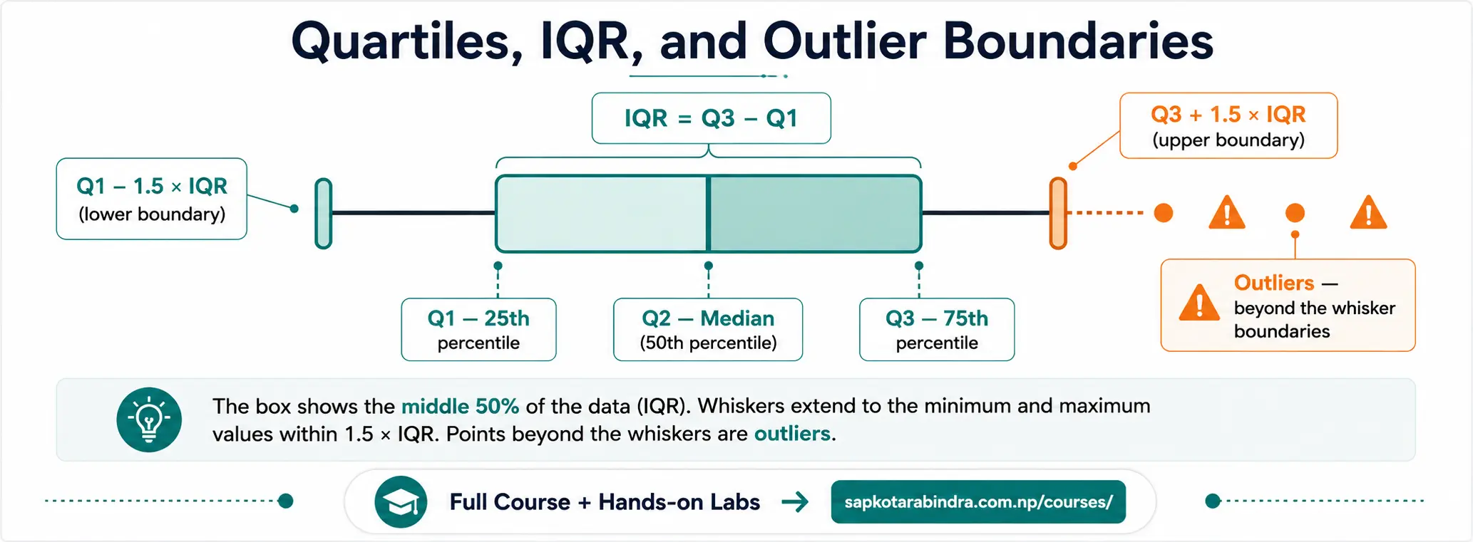
- IQR shows the spread of the middle 50% of the data.
Formula:
IQR = Q3 - Q1IQR is useful because it is not strongly affected by outliers. Detecting Outliers Using IQR Values are often considered outliers if they are:Below Q1 - 1.5 × IQR(lower limit) orAbove Q3 + 1.5 × IQR(upper limit) 📌 IQR helps us find values that are unusually small or unusually large.
Interquartile Range: IQR
6. Dispersion
- Dispersion tells us how spread out the data is. It helps answer: Are the values close together or far apart?
Example:
Dataset A:
[38, 40, 42]Dataset B:[5, 20, 95]Both datasets have mean 40. But Dataset B is much more spread out. That spread is called dispersion. - The common measures are: - Range - Variance - Standard Deviation
- Range is the difference between the maximum and minimum value.
Formula:
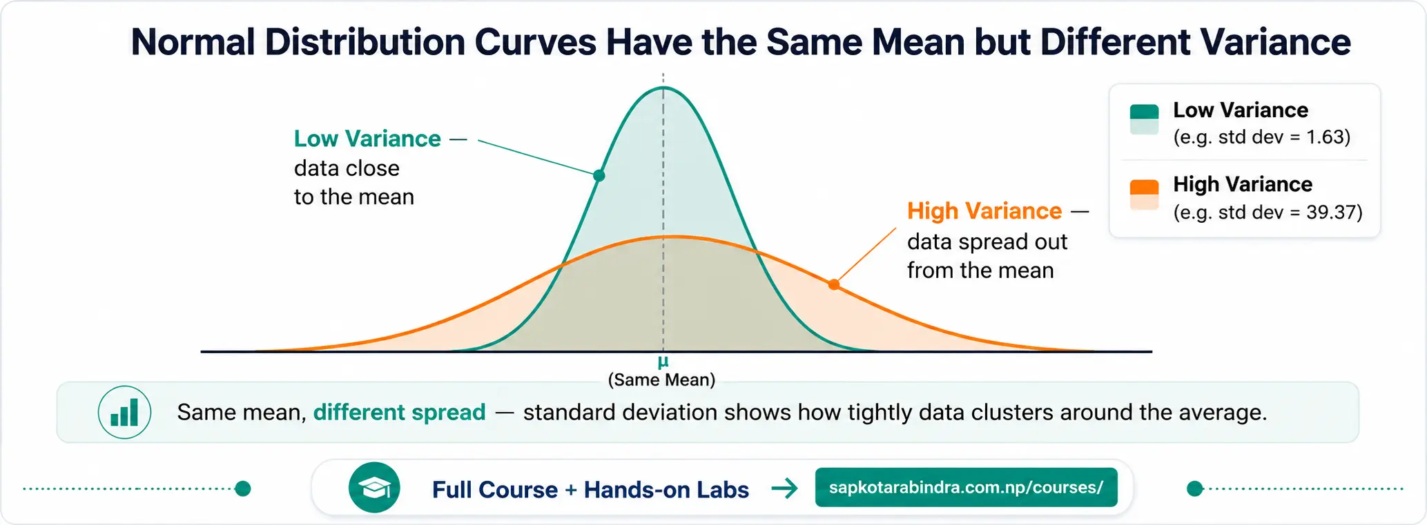
Range = Max - MinExample: For data:[2, 1, 2, 5, 100]Range:100 - 1 = 99So, the range is99. 📌 Range gives a quick idea of spread, but it is highly affected by outliers. - Variance tells us how spread out values are from the mean.
Simple meaning:
- High variance ➜ Values are spread far from the mean
- Low variance ➜ Values are close to the mean
Formula:
Variance = Σ(Xi - X̄)² / N
6.1 📏 What is Dispersion?
6.2 Common Measures of Dispersion
6.3 📐 Range
6.4 📊 Variance
- Standard deviation is the square root of variance.
Formula:
Standard Deviation = √VarianceStandard deviation is easier to understand than variance because it is in the same unit as the original data. 📌 Standard deviation tells us how much values usually differ from the average.
6.5 📉 Standard Deviation
7. Example: Dispersion Calculation
- For data points
[5, 20, 95]: Mean:(5 + 20 + 95) / 3 = 120 / 3 = 40Minimum:5Maximum:95Range:95 - 5 = 90
7.1 Given Data
7.2 Variance and Standard Deviation Calculation
| Value (X) | Difference from Mean (X - X̄) | Squared Difference (X - X̄)² |
|---|---|---|
| 5 | 5 - 40 = -35 | (-35)² = 1225 |
| 20 | 20 - 40 = -20 | (-20)² = 400 |
| 95 | 95 - 40 = 55 | (55)² = 3025 |
| Variance | (1225 + 400 + 3025) / 3 = 1550 | |
| Standard Deviation | sqrt(1550) = 39.37 |
Example showing calculation of Variance and Standard Deviation
8. Covariance and Correlation
- In Data Science, we often want to know how two variables are related. Examples: - Does more study time lead to higher marks? - Does more advertising increase sales? - Does temperature affect ice cream sales? - Does income affect spending? To study relationships, we use: Covariance and Correlation
- Covariance tells us whether two variables move together.
Formula:
Cov(X, Y) = Σ((Xi - X̄)(Yi - Ȳ)) / N
8.1 🔗 Why Do We Study Relationships Between Variables?
8.2 🔄 Covariance
Covariance Types
| Type | Description | Example |
|---|---|---|
| Positive 📈 | Both variables increase or decrease together. | More study time, Higher marks |
| Negative 📉 | One variable increases while the other decreases. | More travel, less saving |
| Zero ➖ | No clear relationship between the two variables. | Shoe Size and Exam Marks |
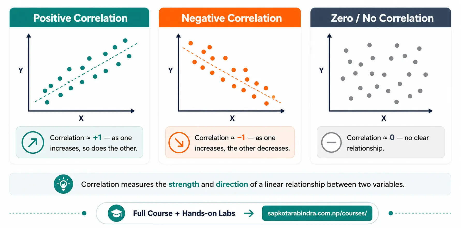
- Covariance tells us the direction of a relationship, but not how strong it is. Correlation tells us both:
✅ Direction of relationship
✅ Strength of relationship
Correlation always lies between
-1and+1. Formula:Correlation = Cov(X, Y) / (Std(X) × Std(Y))
8.3 📈 Correlation
Interpretation of Correlation Values
| Correlation | Meaning |
|---|---|
| +1 | Perfect Positive Correlation: Both variables increase together. |
| -1 | Perfect Negative Correlation: One variable increases while the other decreases. |
| 0 | No or Very Weak Correlation: No clear relationship between the two variables. |
| 0.5 | Moderate Positive Correlation: As one variable increases, the other tends to increase moderately. |
Interpretation of Correlation Values
9. Example: Covariance and Correlation Calculation
X = [5, 20, 95]Y = [10, 30, 50]Mean of X:X̄ = (5 + 20 + 95) / 3 = 40Mean of Y:Ȳ = (10 + 30 + 50) / 3 = 30
9.1 Given Data
9.2 Calculation table of Covariance and Correlation
| X | X - X̄ | (X - X̄)² | Y | Y - Ȳ | (Y - Ȳ)² | (X - X̄) * (Y - Ȳ) |
|---|---|---|---|---|---|---|
| 5 | 5 - 40 = -35 | (-35)² = 1225 | 10 | 10 - 30 = -20 | 400 | (-35) * (-20) = 700 |
| 20 | 20 - 40 = -20 | (-20)² = 400 | 30 | 30 - 30 = 0 | 0 | (-20) * (0) = 0 |
| 95 | 95 - 40 = 55 | 55² = 3025 | 50 | 50 - 30 = 20 | 400 | 55 * 20 = 1100 |
Example showing calculation of Covariance and Correlation
Var(X) = (1225 + 400 + 3025) / 3 = 4650 / 3 = 1550Var(Y) = (400 + 0 + 400) / 3 = 800 / 3 = 266.67Cov(X, Y) = (700 + 0 + 1100) / 3 = 1800 / 3 = 600Std(X) = √1550 = 39.37Std(Y) = √266.67 = 16.33Correlation = 600 / (39.37 × 16.33) = 600 / 642.86 = 0.93📌 Interpretation: Correlation is 0.93, which means X and Y have a strong positive relationship.
Calculations
10. Spearman Rank Correlation
- Spearman Rank Correlation is used when data has rank or order. It is useful for ordinal data.
Examples of ordinal data:
- T-shirt size: S, M, L, XL
- Rating: Poor, Average, Good, Excellent
- Rank in class: 1st, 2nd, 3rd
- Satisfaction level: Low, Medium, High
T-shirt sizes have order:
S < M < L < XL. So, we can rank as:S = 1, M = 2, L = 3, XL = 4Formula:ρ = 1 - (6 × Σd²) / (n × (n² - 1)) T-shirt Size = ['M', 'S', 'L', 'XL']Customer Satisfaction = [3, 4, 2, 5]
10.1 🏆 What is Spearman Rank Correlation?
10.2 Calculation Example
Spearman Rank Correlation for T-shirt Size and Satisfaction
| T-shirt Size | Rank T-shirt (R1) | Satisfaction | Rank Satisfaction (R2) | d = R1 - R2 | d² |
|---|---|---|---|---|---|
| M | 2 | 3 | 2 | 2 - 2 = 0 | 0² = 0 |
| S | 1 | 4 | 3 | 1 - 3 = -2 | (-2)² = 4 |
| L | 3 | 2 | 1 | 3 - 1 = 2 | 2² = 4 |
| XL | 4 | 5 | 4 | 4 - 4 = 0 | 0² = 0 |
Ranking and calculation of Spearman correlation
- The table above shows each T-shirt size and satisfaction score converted into ranks, along with the rank difference (d) and squared difference (d²) needed for the formula.
Calculation
n = 4Σd² = 0 + 4 + 4 + 0 = 8n(n² - 1) = 4(4² - 1) = 4(16 - 1) = 60ρ = 1 - (6 x 8) / 60 = 1 - 48/60 = 1 - 0.8 = 0.2📌 Interpretation: Spearman correlation is 0.2, which shows a weak positive relationship between T-shirt size and customer satisfaction.
Ranking Table
11. Probability
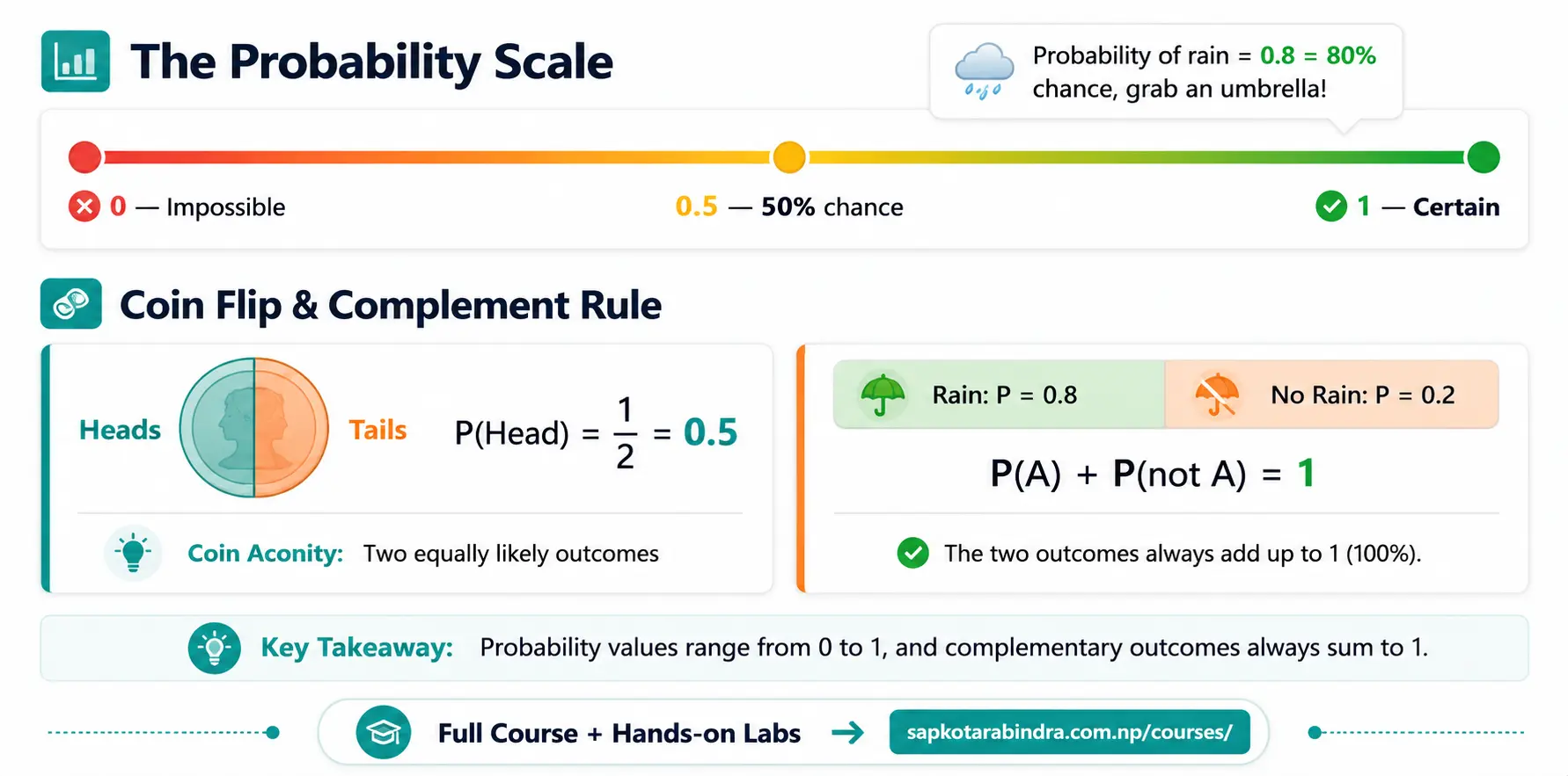
- Probability tells us how likely something is to happen. It is a number between
0and1. Interpretation:0➜ Impossible0.5➜ 50% chance1➜ Certain ☔ Simple Example If a weather app says:Probability of rain = 0.8It means there is an 80% chance of rain, so carrying an umbrella is a smart choice. P(A) = Number of favorable outcomes / Total number of outcomesExample: If a coin is flipped, possible outcomes are:Head, TailProbability of getting Head:P(Head) = 1 / 2 = 0.5So, there is a 50% chance of getting Head.
11.1 🎲 What is Probability?
11.2 Probability Formula
- Rule 1: Event and Not Event
P(A) + P(not A) = 1Example: If probability of rain is 0.8:P(no rain) = 1 - 0.8 = 0.2Rule 2: A or BP(A or B) = P(A) + P(B) - P(A and B)This is used when we want either event A or event B to happen.
11.3 Basic Probability Rules